Logic will get you from A to B. Imagination will take you everywhere. —Albert Einstein
Logical data model
In this chapter, we introduce the concept of a ‘database model’ as an introduction to building the logical data model. Then, we can make the conversion from the conceptual to the logical data model. We will take a look at:
- What is a database model?
- What is the role of a database model?
- What is the relational database model?
- How to convert a conceptual data model to a logical data model according to the relational database model?
You should be able to define the following terms, how to visualize this (where relevant) and explain with an example:
- logical data model;
- database model;
- relational database model;
- table;
- key (including candidate key, primary key, foreign key, composite key, natural key, technical or surrogate key)
- normalization.
After completing this chapter, you should be able to read the notation of a logical data model (of a relational database model) and explain it using an example.
You should also be able to Convert a conceptual data model to a logical data model (of a relational database model).
Introduction
After the conceptual data model, we move on to the design of our database. We had described a database as a collection of "persistent data". To determine what specifically should be included in that collection, we created the conceptual data model that addressed the question ‘What information should we include in our database’. In doing so the collection is delineated to a particular topic or application. An example of this is the UCLL College student administration database, with data of students, programs, enrollments, ...
In the next step, we will consider the structure of this collection of data. How do we organize the data? After all, there are several ways to do that.
Before we focus on the different ways in which we can apply structure, we should take a moment to consider the question ‘Why is structure important?’. When we work with computers, structure ensures that we can teach these computers to work within the framework of this structure. Structure in itself provides predictability so that it becomes easy to define procedures on it. This is by the way, not only the case for computers: the fact that there are markings on the roads structure the roads in such a way that rules can be defined that promote road safety. And we are all happy about that.
For data, this gives the added benefit that the structure itself contains additional information (we call this metadata - data about the data) that can then be used to determine procedures. Thus we can manage data access, optimize storage, develop standard procedures, ...
You can structure the same concept in a lot of different ways, just think of a library. You can arrange all the books by theme, by author, by title, ... This is no different for data. You then ask the following questions:
- what type of data are we talking about?
- what do you want to do with this data?
Because IT people are rather fond of standards (and you future IT guys should be getting excited by now because a standard is clearly coming), it should come as no surprise that this is also the case for data. A lot of standards have been defined over time for data models and to structure data. We call these standards database models.
Database models
A database model defines the structure of a database and how the data within a database is organized and manipulated. Let's take a look in a little more detail.
First and foremost, a database model will structure data in a specific way. This typically involves the use of a number of components or building blocks, each of which play a role in the structure of the data model. That role is then typically described by a number of principles or rules that define the cooperation of the various components.
The standards around database models (and other domains) provide some important advantages that we should not lose sight of:
- First and foremost, these are standards used across the industry . When you talk about a particular standard, everyone around the table with an IT training understands what you are talking about. This also applies to database models.
- A second advantage is that a lot of researchers continue to work on these standards and additional extensions (like the EERD). They continue to develop procedures that benefit everyone, so standards typically do continue to evolve. It's your job to keep up. Lifelong learning ...
- A third benefit is that the standards provide a foundation for companies to develop software products. Since they are based on standards, they can in turn work well with other products that in turn also use standards.
Over the years, many different database models have been developed. Some have been developed from particular technologies. Others to work with new types of data. Others because the development of ever more powerful machines expanded the possibilities of working with data. In short, the horizon of what is possible is constantly expanding, and so does the range of database models available.
Of all these database models, one particular database model has been going for a long time. The relational database model, developed in the 1970s by Codd, is still considered a standard within the IT industry. Within this course, this is therefore the database model on which we will focus further. Some others are covered in other courses.
Relational database model
Table
The relational database model uses only one component or building block, the table. All the data we want to track, will be put into one or multiple tables. Each table represents a collection of similar data, for example, a table containing all student data. A table is structured as a 2-dimensional array structure, where we call the horizontal dimension the rows and the vertical dimension the columns.
A row represents a record (or entity) of the table. A table can theoretically contain an infinite number of rows. As we create a table with student records, each row might represent a student.
A column represents an attribute (or field) of the table, each of which will describe a piece of the row (or entity). A table contains a fixed number of columns. If we want to add a column, which is possible, then we need to think what this means for the existing rows in the table. For example, it is possible that we need to enter a value for this column for each of the rows already included in the table.
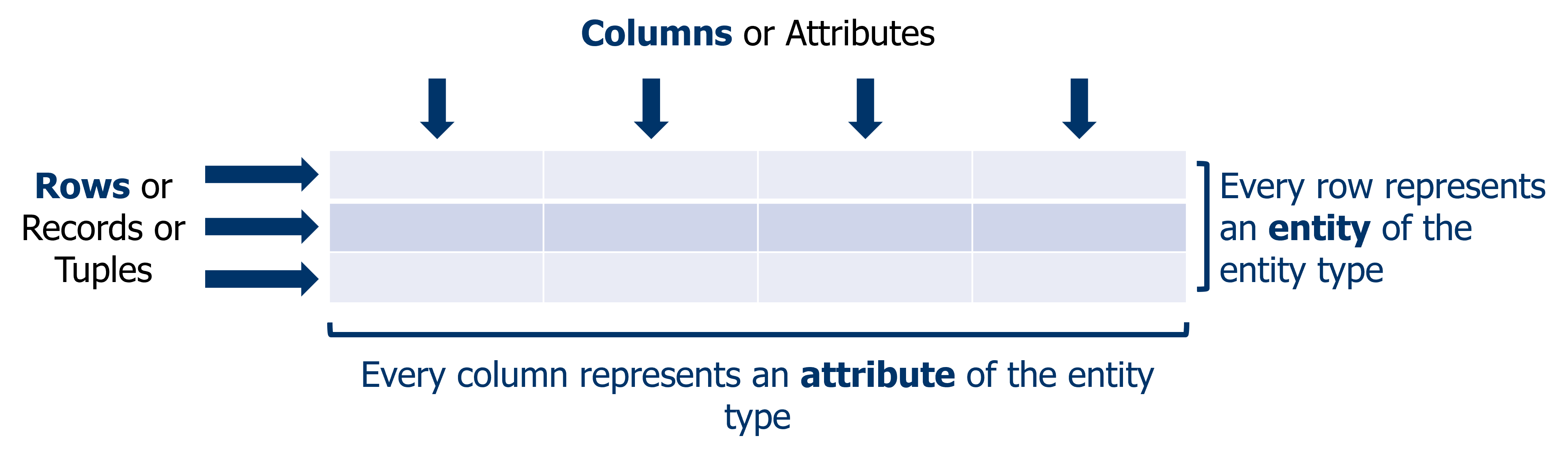
In our example of a table of student data, each column would contain a certain property of the student, for example, the name, the birthdate, ...
Therefore, because a table has a specific structure of columns, also all data maintained in one table will always have the same structure. Every time we want to keep additional data with a different structure, we create an additional table. In a relational database model, we call a set of a number of tables "a database". So our relational database can contain many different tables. To then combine these tables with each other and create relationships, we use keys.
Keys
A key consists of one or more columns (attributes) of a table that satisfy the following three conditions:
- The value of the combination of one or more columns in a row constitutes a unique identifier of the entire row. Thus, for each row, the value of the key must be unique; in other words, two rows in the table must not have the same key.
- The combination of the columns forming the key must be minimal. By this we want to indicate that if in the combination we were to remove one of the columns, we would no longer satisfy the first condition. If we have a key consisting of one column, our key is minimal by definition.
- The value of the key may also not be empty, the key must thus always be filled in.
Within the relational model, we define one primary key for each table . The value of the primary key is a unique identifier for each row. We will use this primary key to connect the different tables with each other.
The primary key is chosen from a number of candidate keys. A candidate key is a potential key for a table, which therefore also satisfies the three conditions for a key.
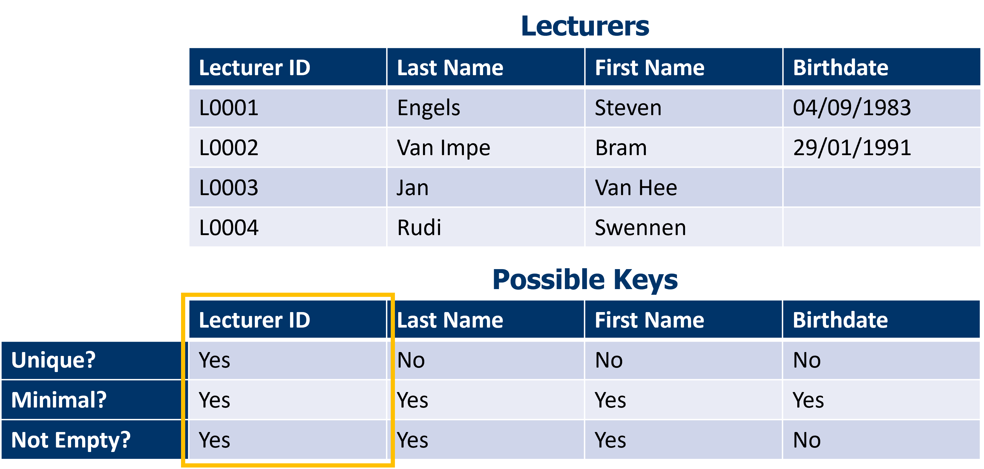
The image below shows an example for the table ‘Lecturers’. We have four columns that might be a key. After consideration we are left with only ‘Lecturer ID’ as a candidate key. Since there is only one candidate key, it makes sense to choose this as the primary key.
So a table can have multiple keys. From the list of candidate keys, we choose one primary key. To choose a good key from the list of possible keys you can consider the following criteria:
- A key should be as stable as possible. In fact, we assume that a key is actually never modified. There are some exceptions to this, but we try to avoid changing a primary key. For example, if within the context of student administration you have the choice between a state registry number or a student number to uniquely identify a student, you choose the student number. Not only do we have within student administration more control over the student number, we can ensure that it is never altered. A state registration number can change. In addition, the use of a national registry number in a database (and outside of it) is subject to very strict GDPR legislation, but we'll explain that in another course.
- A key ideally includes as few columns as possible. Keys can consist of one or more columns. A key that consists of multiple columns, is called a composite key simply because it is composed of multiple values. We avoid compound keys because that makes the whole thing a bit more complex, and complexity brings a cost that we try to avoid. Complexity means that the whole is difficult to understand for the parties involved, that there is possibly a loss of performance when processing the data, etc. As soon as you learn about performance, automation, security, ... we will be able to explain the cost of complexity in a database.
- A key is ideally a simple value, for example a number or a short sequence of characters. As soon as it becomes more complex, or even starts using special characters, the risk of errors increases.
- A key is ideally taken from the context that we are describing. A key that is both valuable within the database (as a primary key) but also used outside the system, has the advantage that a lot of the people involved quickly understand what it is about. For example, a student number is also a way to identify students outside the database. So student number is potentially a good primary key. A key that is used both within and outside the database, is called a natural key.
If we have no candidate keys, or the available candidate keys are not a suitable choice, we always have the option to define a key ourselves. We call those technical or surrogate keys. The technical key is only used inside the database, and has no value outside the database. It has the effect of adding an additional column that will contain the key. Ultimately, each table must have a primary key.
We had already indicated that primary keys make it possible to create links between tables. This is done by an exchange of primary keys. The mechanism of the exchange is explained in the section ‘From conceptual to logical data model’. Essentially, the primary key of one table is added to another table. As soon as we add a primary key to another table, and thus add a column to that table, we call this key a foreign key.
The use of primary keys and foreign keys is central in the relational model. It is the basis for defining relationships.
Other database models
In addition to the relational database model, there are many other database models, each with their specific applications. Some of these database models have found their way into certain technologies so that a good understanding of the model should enable you to understand the operation of the technology as well. We will discuss this in more detail in other courses but to give you a foretaste, we have already listed some database models:
- Hierarchical database model: uses tree structuring to represent data
- Network database model: uses network structuring to represent data
- Dimensional database model: used in the context of data warehouses
- Object-oriented database model: combines the capabilities of a relational db with object-oriented programming
- Graph database model: uses graph structuring to represent data
From conceptual to logical data model
How to draw a logical data model in draw.io can be found in a separate chapter in two videos:
The logical data model answers the question ‘How should we structure the data according to our chosen database model?’ We developed a conceptual data model, and made the choice of a relational database model. The conversion of this conceptual data model then proceeds in a number of steps.
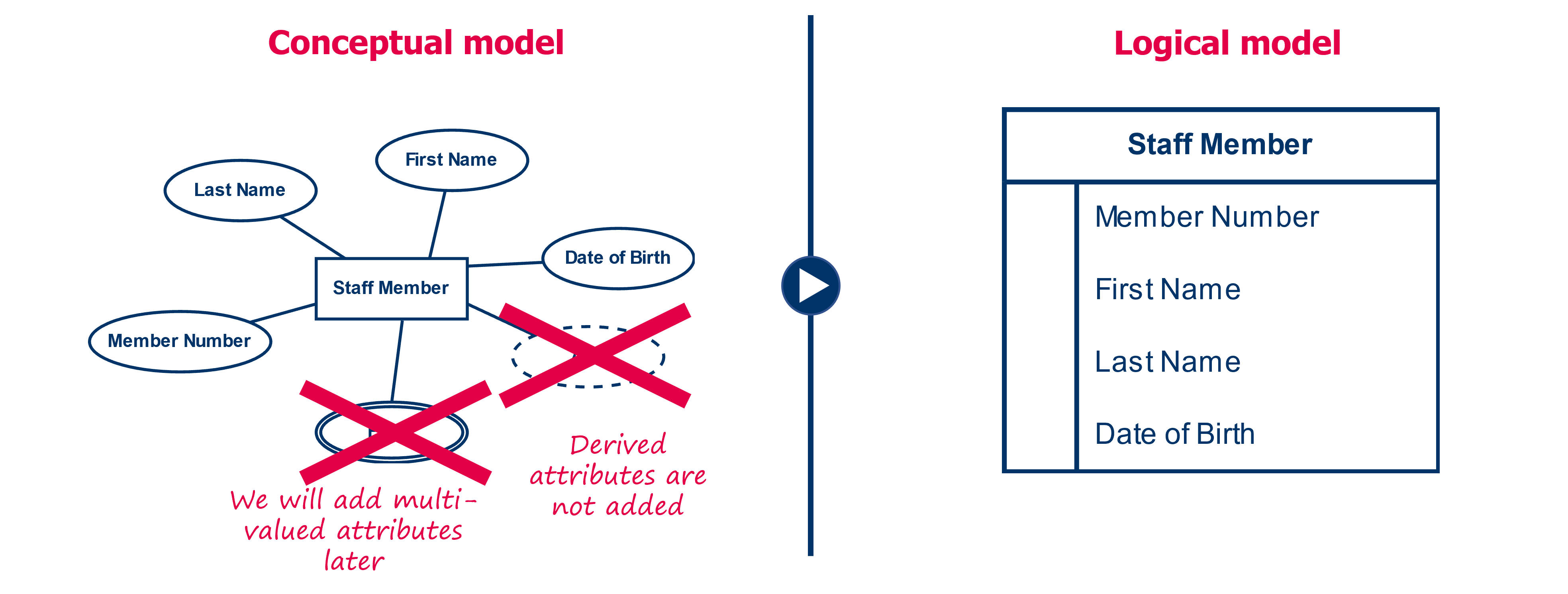
Step 1: entity types become tables
In the first step, we create a table for each of the entity types. We give this table the same name as the entity type. Then we define the columns of the table, creating a column for each attribute , except for the multi-valued attributes and the derived attributes. We will come back to the multi-valued attributes later. The name of the column created matches the name of the attribute.
The notation of the logical data model is different from that of the conceptual data model. We represent the whole of a table as a frame, containing a list of its attributes.
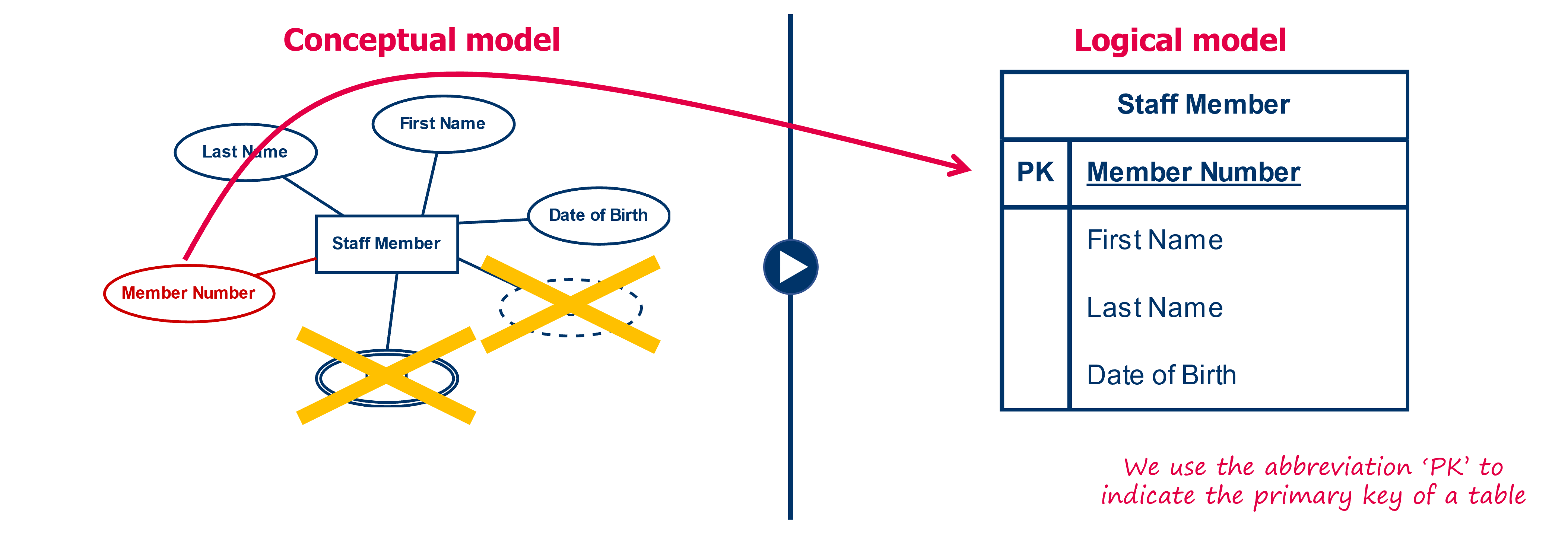
Step 2: each table is assigned a primary key
In a second step, we designate a primary key for each table. This means that we need to determine a number of candidate keys and from this list then select the best candidate.
We visualize the primary key by placing the columns of the key at the top of the list with a line below to clearly distinguish between the primary key and the remaining columns. In doing so we also put for the different columns of the primary key the code ‘PK’ (from primary key) and to be completely sure that nobody can make a mistake, we underline the column names as well.
We do this for each table. Also keep in mind that you may create a technical key, if it is difficult to create a primary key with the existing columns.
Step 3: for each 1-1 and 1-N relationships, we transfer the primary key as a foreign key
In the third step, we are going to convert some of the relationships from the conceptual data model to something equivalent in the logical data model . Since we create relationships within the logical data model by means of keys, we are going to work with primary and foreign keys.
For each 1-N relationship, we're going to transfer the primary key from the 1-side to the N-side. On the N side, this primary key then becomes a foreign key. So each row of the table on the N-side will get an additional column containing a reference (by means of the foreign key) to a row in the 1-side table.
For example, we have two entity types: ‘Team’ and ‘Staff Member’. Each staff member is in exactly one team. Each team can include multiple staff members. We create two tables: a table ‘Team’ and a table ‘Staff member’. The table ‘Team’ is given the primary key ‘Team Code’, by which every team in the table gets a unique team code. The table ‘Staff member’ is given the primary key ‘Member number’, by which every staff member in the table is assigned a unique member number. In order to model the relationship between the two entity types in the logical data model, we append the team code from the ‘Team’ table (1-side) to each staff member in the ‘Staff Member’ table (N-side).
The reverse (i.e., adding the primary key from ‘Staff Member’ to ‘Team’) is not an option. We can add only one value to a team. Thus, if we were to make a reference from the team to one staff member, we would lose the connection to the other team members of the team.
In the data model we add the foreign key to the list of columns. We denote the foreign key by the abbreviation "FK" (from foreign key) followed by a sequence number, for example FK1, FK2, ... The sequence number should make it possible to distinguish the different foreign keys from each other. If we have a foreign key that consists of multiple columns, we transfer each of the columns. We then give them all the same sequence number to indicate that they belong together.
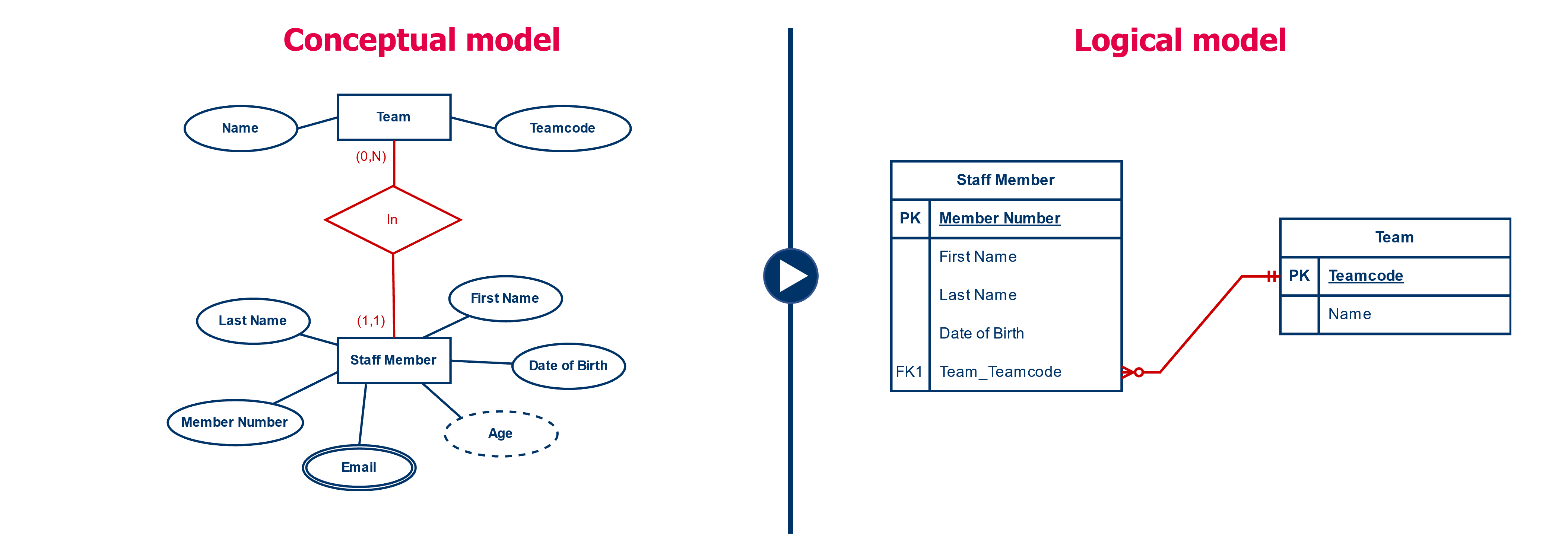
We still denote the relationship by a line where we use the crow's foot notation. The crow's foot notation is different from the (min,max) notation you have used so far.
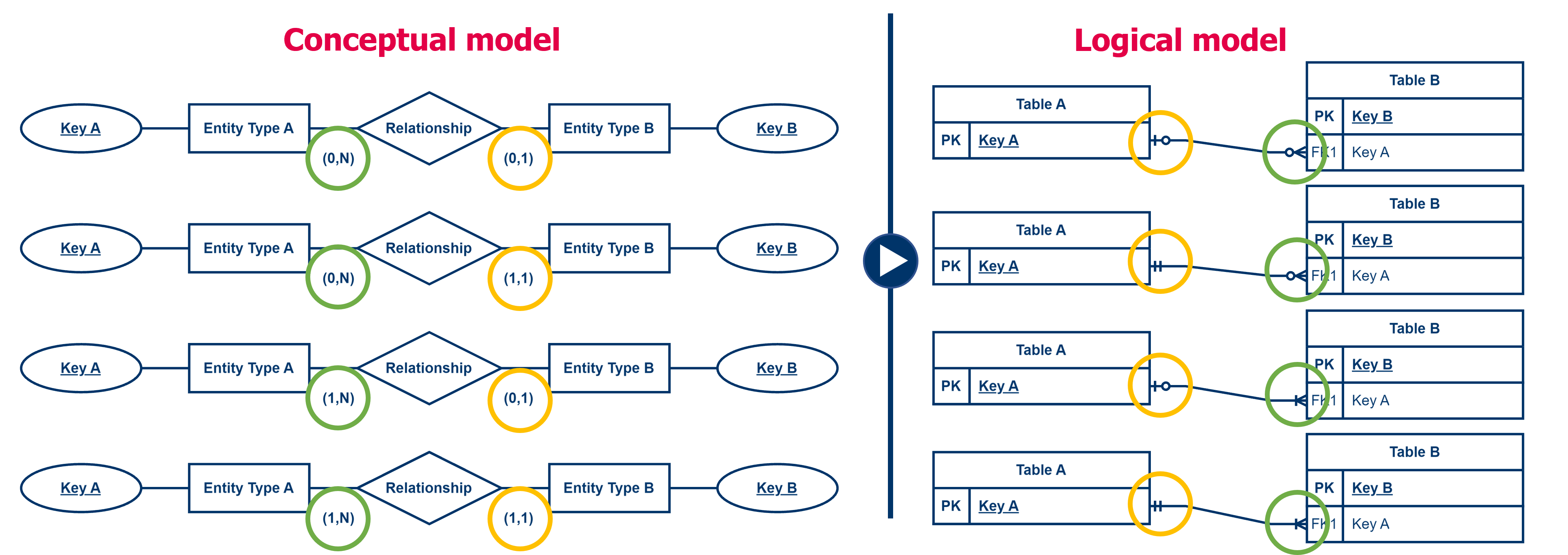
For each of the 1-1 relationships, we do something similar, only here we can choose from which side we take the primary key to add to the other side as a foreign key.
The guideline with a 1-1 relationship is to look at the minimum cardinality. If a given entity type cannot exist without the relationship (so minimum cardinality is ‘1’), this table best takes the primary key of the other table as the foreign key. Since an entity only exists if it has a relationship, then the row describing the entity must always have this value filled in. Because without this value, the relationship does not exist.
If both entity types cannot exist without each other (both thus have a minimum cardinality of ‘1’), or both can both exist without each other (i.e., both have a minimum cardinality of ‘0’), you may choose. Typically, you then choose the table with the smallest number of rows to include the primary key of the other table as the foreign key.
Multi-valued attributes
Multi-valued attributes are a type of 1-N relationship where an entity is related to multiple attribute values . Therefore, you need to use a similar approach for these as for converting 1-N relationships. For each multivalued attribute, create a new table named with the name of the multivalued attribute. To this table you add the value of the attribute and then the primary key of the entity type table as the foreign key. Don't forget to indicate the primary key and to add a line in crow's foot notation.
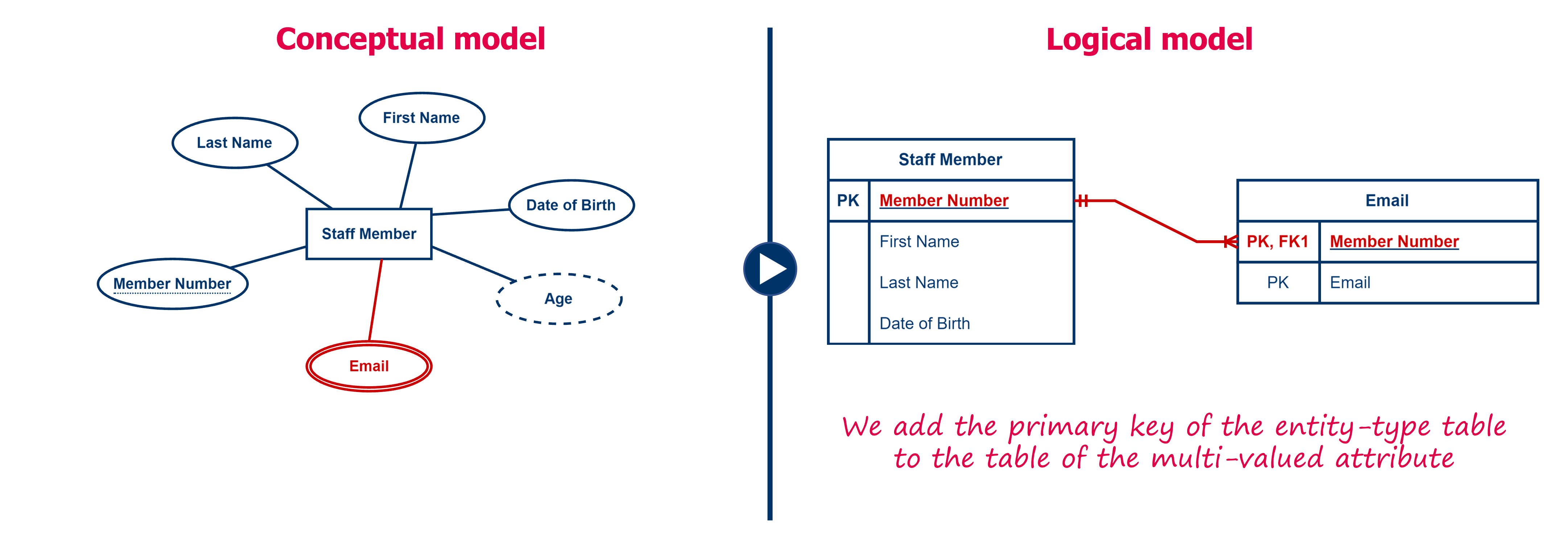
For example, the multi-valued attribute ‘Email’ of the entity type ‘Employee’ results in a table ‘Email’ containing a column ‘Email’. To associate each email address with a staff member, we add the primary key of the table ‘Staff member’ as a foreign key to the ‘Email’ table. Note in this example that the primary key of the table ‘Email’ is a composite key: only the combination of the columns ‘Staff Member’ and ‘Email’ is unique.
Step 4: For each N-M relationship, we create an intermediate table
Now things get a little more complex.
In the paragraphs above, we already gave a procedure for the different entity types, their attributes and for the 1-1 and 1-N relationships. In this step we focus on the N-M relationships. To enable N-M relationships, we need to go beyond the simple exchange of primary keys because this does not provide a good solution for N-M relationships.
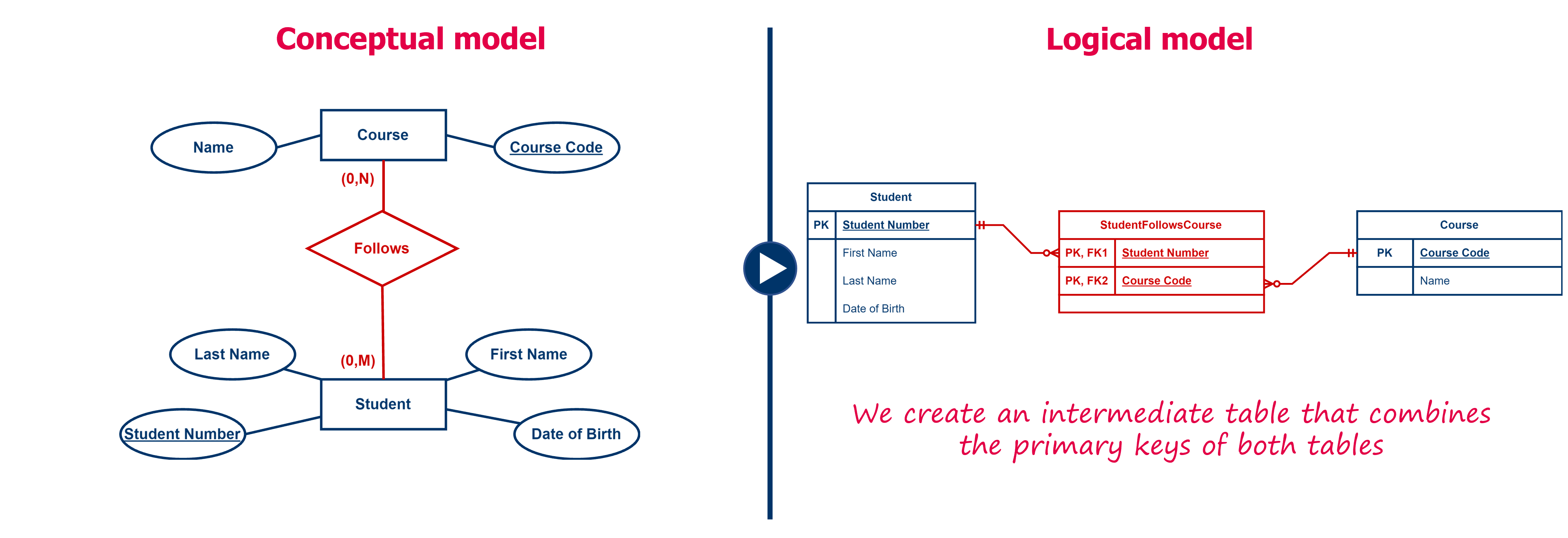
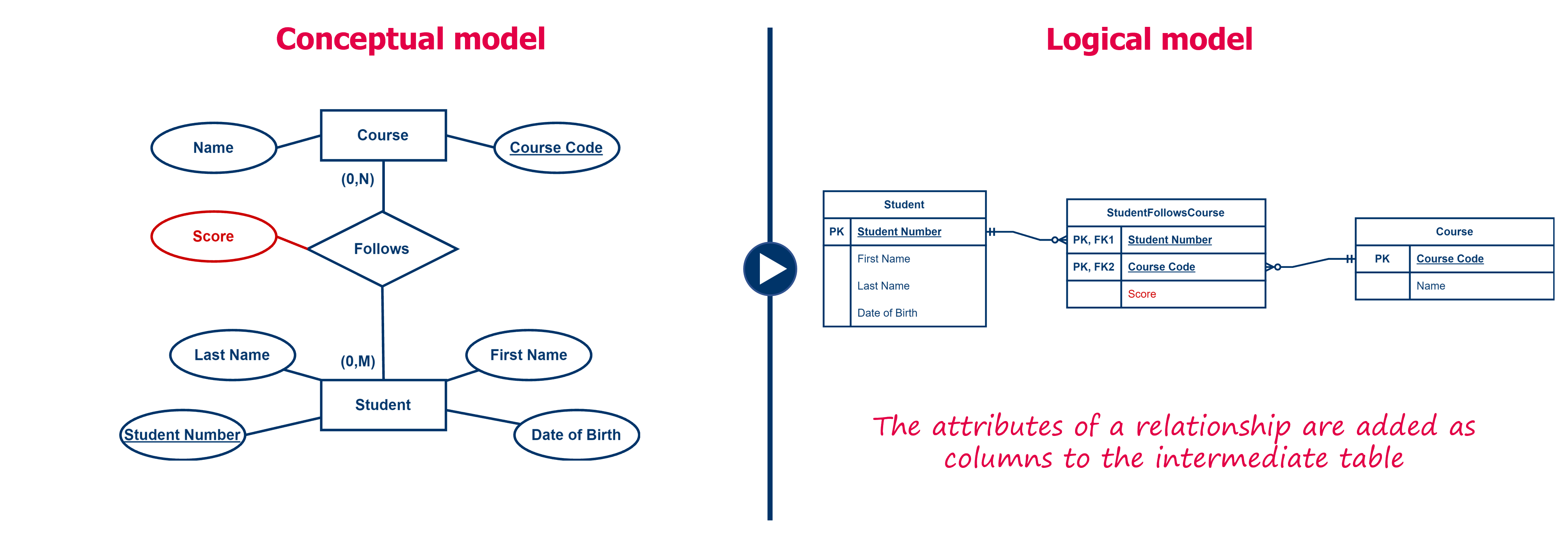
Let's start from an example. We have the entity type ‘Student’ and the entity type ‘Course’. Between both entity types we have a relationship that expresses that a student can enroll in multiple courses, and conversely that in a course multiple students can enroll. So this is a many-to-many relationship.
Initially, we create two tables from both entity types: the ‘Student’ table and the ‘Course’ table. The first table gets as primary key ‘Student Number’, the second table gets as primary key ‘Course Code’. If we were to add the ‘Course Code’ column to the table ‘Student’, a student could refer to only one course and thus could take only one course, which is not correct. Conversely, should we add the ‘Student Number’ to the ‘Course’ table, a course could only be taken by one student, which is also not correct.
We solve this by creating an intermediate table, to which we add a row for every combination of a ‘Student’ entity following a ‘Course’ entity. Each row then contains the primary key of the table ‘Student’ and the primary key of the ‘Course’ table. Thus, the table will contain two foreign keys. The combination of the two foreign keys, will then become the new primary key of the new intermediate table.
The same rules we gave earlier for a key also apply here. So if there is a need for multiple relationships between the same two entities, the combination of the foreign keys might be insufficient to satisfy all the rules. That means something might be missing in your data model.
In other words, the above example results in an (intermediate) table ‘StudentFollowsCourse’ (or ‘Student_Course’, be consistent in your naming) in which we find the ‘Student Number’ column and the ‘Course Code’ column. Both are foreign keys, so we denote them with the abbreviation ‘FK’ (Foreign Key) followed by a sequence number. The combination of both keys is also the primary key of the new table, so we denote each column also with abbreviation ‘PK’ (Primary key). Study the figure below carefully!
An N-M relation is the only type of relationship that can have attributes. In a logical data model, we are going to create additional columns for these attributes in the intermediate table
For example, in the above example, if we want to keep a score for each combination between student and course then we create an additional column ‘Score’ in the table ‘StudentFollowsCourse’ (see figure below).
Step 5: the special cases
There remain some constructs in the conceptual data model that we have not yet given a solution for. We want to explain them briefly so that you can also convert these from a conceptual to a logical data model.
Relationships of degree 1
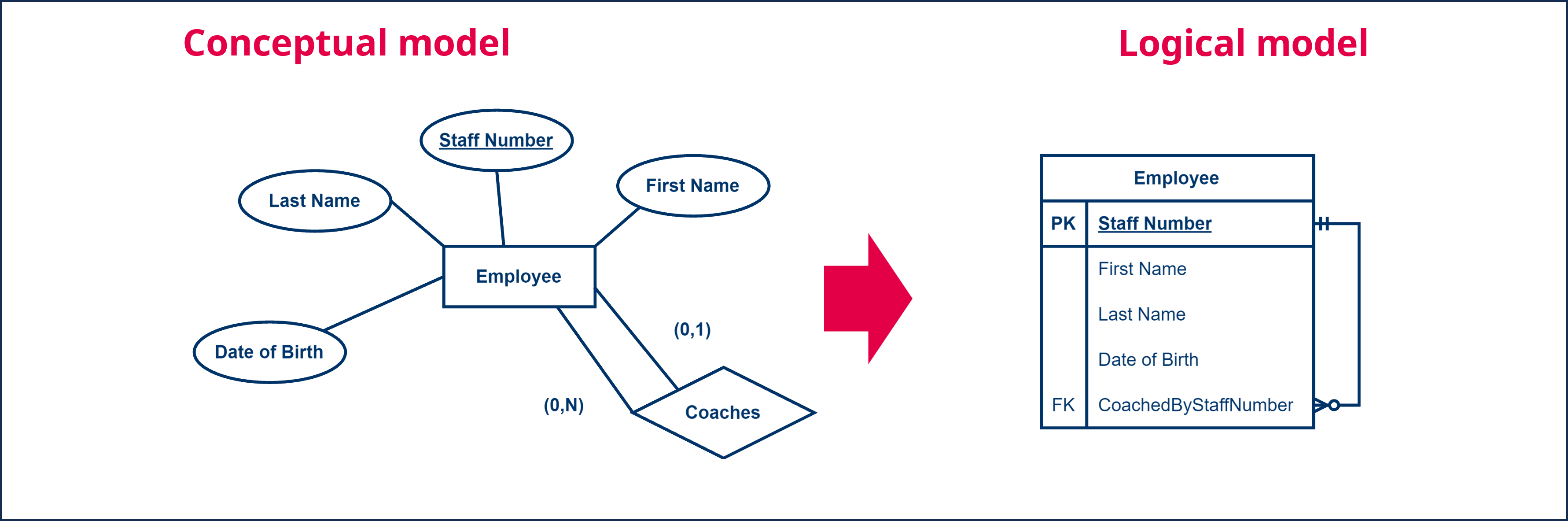
A grade 1 relationship in a conceptual data model, also called an unary relationship, is a situation in which an entity type has a relationship with itself.
For example, consider a situation where an employee is coaching another employee. We want to include this information in our database (and therefore in our data model). We have an entity type ‘Employee’ that refers to itself via a relation ‘Coaches’. The relation specifies that each employee possibly coaches several other employees or none. In addition, each employee has at most 1 coach, but again this is not mandatory.
To then convert this into a logical data model, we treat this unary relationship as if it were a binary relation, corresponding to a 1-N relation.
How do we approach this practically? First, we create a table ‘Employee’ and define a primary key, in this case ‘Staff Number’. In the situation of a 1-N relationship, we carry the primary key from the 1-side (coaching employee) as a foreign key to the N-side (coached employee). We add the primary key ‘Staff Number’ as an additional column to the table ‘Employee’ where we rename it ‘CoachedByStaffNumber’ for clarity and we designate it as a foreign key with the abbreviation ‘FK’, optionally followed by a sequence number. This allows us, for each employee, to connect to his or her coach because each row of the employee will contain a reference.
For the other types of relationships, the reasoning runs similarly. If a unary relation is an N-M relation, we use an intermediate table as described earlier.
Relationships of degree 3 and higher
A relationship of degree 3 and higher in a conceptual data model is a situation where a relationship connects three or more entity types.
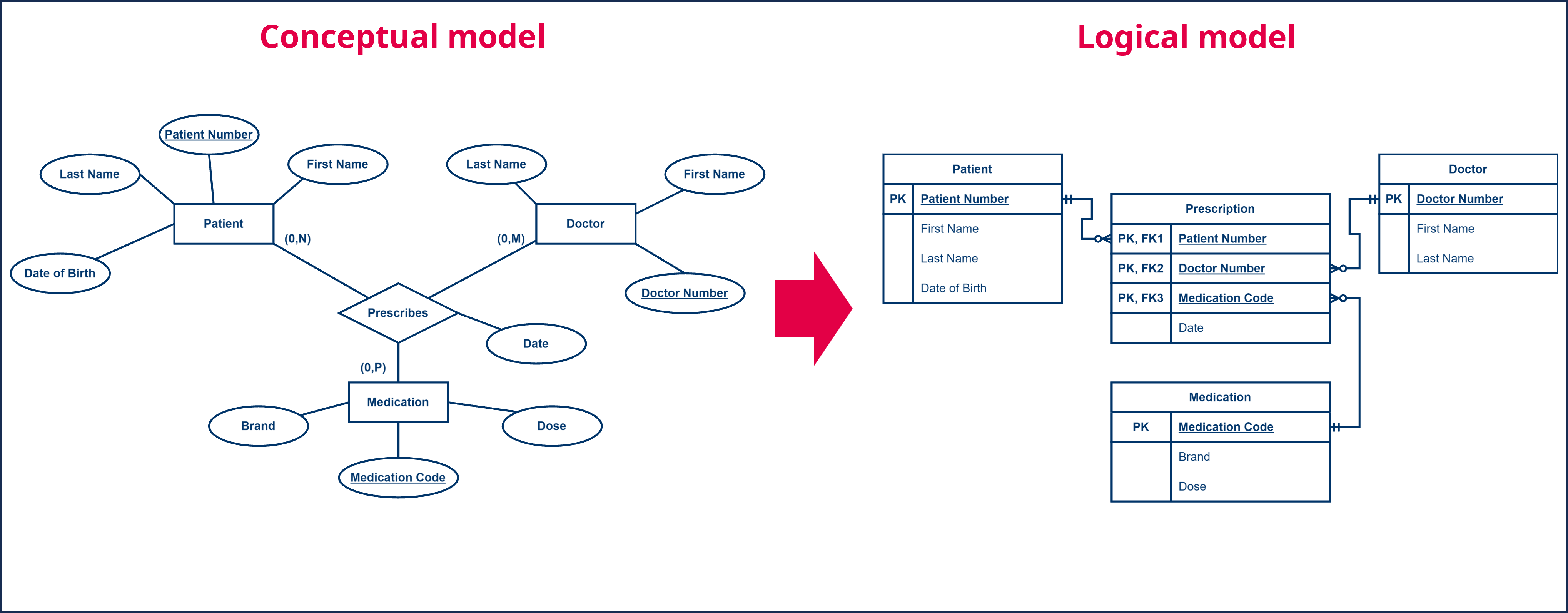
For example, imagine a situation where a doctor prescribes medication to a patient. If we model this in a conceptual data model we would have three entity types ‘Doctor’, ‘Patient’ and ‘Medication’ that are connected by a relationship ‘Prescribes’. We have previously used this example in the chapter of the conceptual data model, so we know we can't reduce this to binary relationships.
To then convert this to a logical data model, we create a table for each of the three entity types: ‘Doctor’, ‘Patient’ and ‘Medication.’ These three tables each have a primary key, ‘Doctor Number’, ‘Patient Number’ and ‘Medication Code’ respectively. We replace the relationship with an intermediate table ‘Prescription’, to which we add the three columns that each refer to the primary keys of the ‘Doctor’, ‘Patient’ and ‘Medication’ tables. Each key is a foreign key in the ‘Prescription’ table and so we denote them with the abbreviation ‘FK’ followed by a sequence number. The three columns together form the primary key of the table ‘Prescription’ and thus we also denote them by the abbreviation ‘PK’. For every relationship that exists between the different entities of the entity types ‘Doctor’, ‘Patient’ and ‘Medication’, a row will be added to the ‘Prescription’ table.
Each attribute of the relationship, for example the attribute ‘Date’ to indicate when the medication was prescribed, is added to the intermediate table ‘Prescription’ as an additional column.
We can extend the same principle for relationships of degree 4, 5, ... In each case, we create an intermediate table that contains the primary keys of all tables involved.
Exercise Car Rental
Create Exercise 1: car rental.
Exercise youth association
Create Exercise 2: youth association.
Exercise board game association
Create Exercise 3: board games association.
Exercise technical maintenance and repair
Create Exercise 4: technical maintenance and repair.
Subtypes and supertypes
We have previously described how the ERD was extended to the EERD, including the ability to create subtypes and supertypes. A subtype is an entity type that inherits attributes and relationships from a supertype and then extends it with additional attributes and relationships. Similarly, we saw that a supertype can have multiple subtypes, each of them a specialization of the supertype.
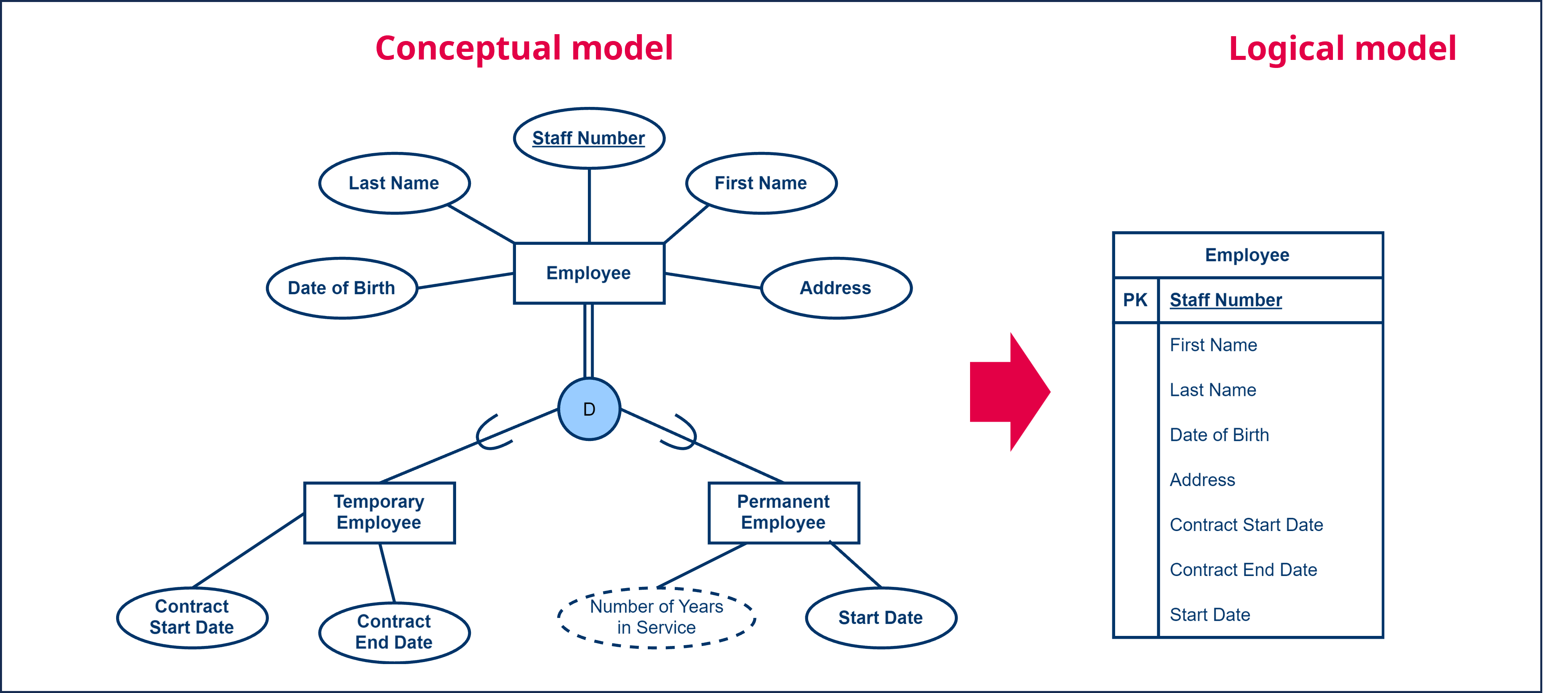
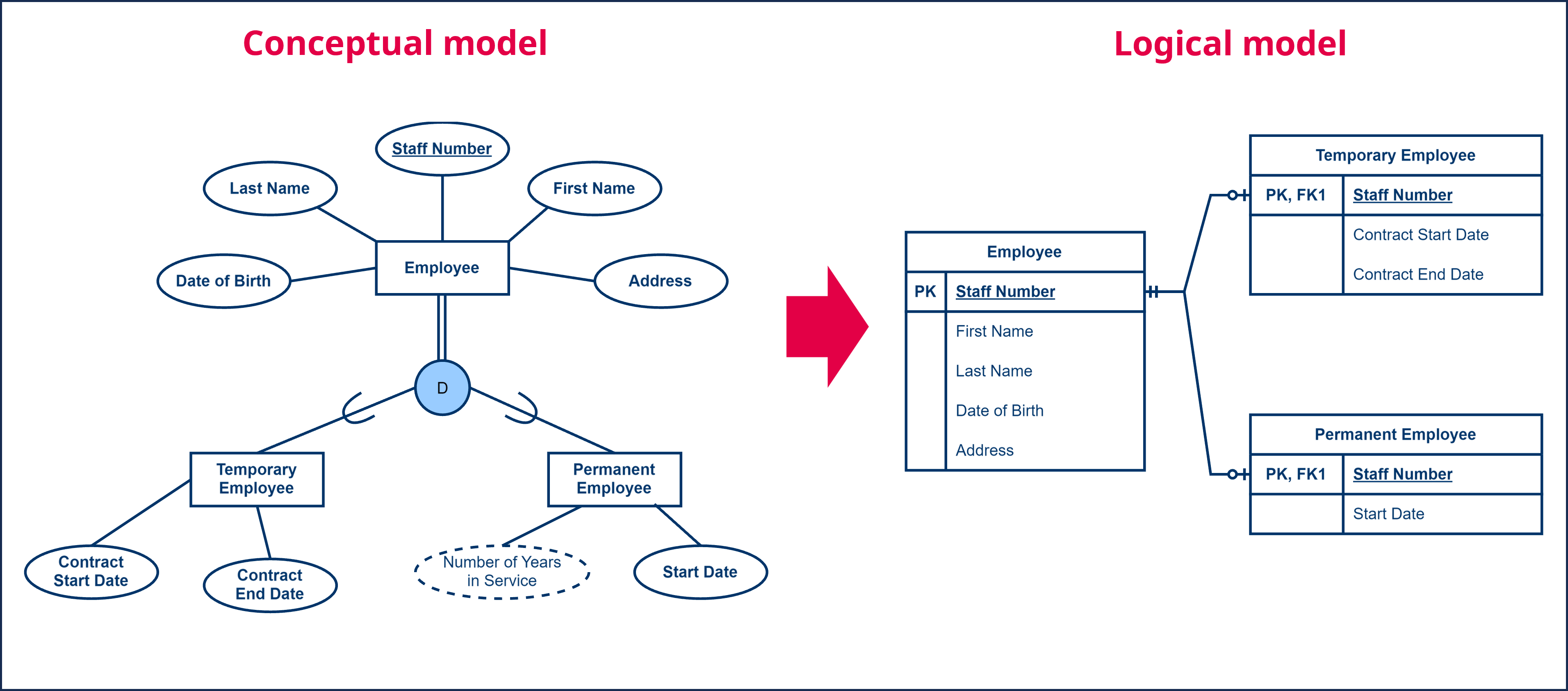
The example we used earlier was a supertype ‘Employee’, and two subtypes ‘Temporary employee’ and ‘Permanent employee’. Of the entity type ‘Employee’, we keep the typical properties: name, first name, date of birth, employee number, ... In addition, we have the entity type ‘Temporary employee’ that inherits all the attributes and relationships from the entity type ‘Employee’, but extends it with the attributes ‘Contract start date’ and ‘Contract end date’. The entity type ‘Permanent employee’ extends the entity type ‘Employee’ with the attributes ‘Employee start date’ and ‘Number of years of service’.
To then convert this to a logical data model, we can use different strategies. The tradeoff between the different strategies is typically done based on performance, and since this course does not focus on performance, you can freely choose your strategy. However, you must be able to apply both strategies.
We'll go over the two strategies:
-
A first strategy is to create one table ‘Employee’, where for each attribute of the entity type ‘Employee’ we add a column, with the exception of the multi-valued and derived attributes. We give this table a primary key, for example, ‘Staff Number’. Then for each of the attributes of the subtypes of the entity type ‘Employee’ (in other words the entity types ‘Temporary Employee’ and ‘Permanent Employee’) we also add columns. This results in one large table with all the attributes of both the supertypes and subtypes. If the subtypes also have relationships, each of the relationships must of course also be added to the table correcty as we described earlier. The resulting table contains one row for every employee, the different columns are filled-in according to whether the employee is a temporary or permanent employee.
This strategy works very well if the supertype contains the largest proportion of attributes and relationships, and the subtypes have only a few additional attributes or relationships each. Thus, we deliberately choose not to add complexity by adding additional tables.
Additionally this strategy works well with overlapping and/or total inheritance . With overlapping and/or total inheritance, we are going to have more attributes filled-in for a given entity, or translated to the logic model, fewer columns will be empty for a given row.
-
A second strategy is to create a single table ‘Employee’, where we add a column for each attribute of the entity type ‘Employee’, with the exception of the multi-valued and derived attributes. We give this table a primary key, for example ‘Staff Number’. We then create additional tables for each of the subtypes, which for our example results in the tables ‘Temporary Employee’ and ‘Permanent Employee’.
To these tables we add a column for each attribute of the subtypes, again with the exception of the multi-valued and derived attributes. To each of the subtype tables we add the primary key of the supertype table. In our example, we add the ‘Employee Number’ column to the ‘Temporary Employee’ and ‘Permanent Employee’ tables. Given that this is the primary key of another table, we denote it as a foreign key with the abbreviation ‘FK’ followed by a sequence number. At the same time, this key also assumes the role of primary key for the subtype tables, so we denote it also with the abbreviation ‘PK’.
This results in several tables, one for the supertype and one for each of the subtypes. Of course, also here the different relationships must be processed correctly as we described earlier. The resulting supertype table contains one row for each employee. In addition, for each temporary employee a row will be added to the table ‘Temporary Employee’. and for each permanent employee a row will be added to the ‘Permanent Employee’ table with each column being filled in accordingly.
This strategy works very well if the supertype includes a small number of attributes and relationships, and the subtypes themselves have a lot of attributes or relationships. To avoid the complexity of all those additional columns that would usually be empty in a single table we split the whole thing up.
Additionally, this strategy works works well if it involves disjoint and/or optional inheritance . With both disjoint and/or optional inheritance, we have a high risk of a lot of empty columns for a given row, which then in turn takes up unnecessary space.
Finally, you can start combining the above strategies, where you create an additional table for certain subtypes, and include other subtypes along with the super-type table.
Exercise library
Create Exercise 5: library.
Redundancy in a relational database model
In the previous section, we briefly touched upon the concept of redundancy. Redundancy means that we are keeping multiple instances of the same information in our data model. For the conceptual data model, this means that when defining entity types, attributes, and relationships, we must be careful not to add logic that is already contained in the data model.
In the context of a relational database model, redundancy means that we define tables and columns that we don't actually need. But how does this look?
Let's start from the example we used earlier. A customer buys a car from one of the garages. We know which customer buys which car. We also know in which garage a car is sold. If we want to know in which garage a customer buys a car, we can establish the relationship ‘Buys car in’ between the entity types ‘Customer’ and ‘Garage’. We mentioned earlier that this relationship is redundant, because the information we can derive from this relationship is already contained in the relationship ‘Buys’ between the entity types ‘Customer’ and ‘Car’ and the relationship ‘Is in’ between the entity types ‘Car’ and ‘Garage’. What would it now mean for our logical data model if we add the relationship anyway?
Based on the above, we might arrive at the following conceptual data model. We have added cardinalities and additional attributes.

If we translate this data model into a logical data model, we get the result below.

Now there is redundancy. Because if we want to know which customer bought a car in a particular garage, we can look at the table ‘Buys_car_in’. We can also look in the table ‘Car’, because for each car sold, there is a reference in this table to both the customer and the garage. But why is this a problem?
When we represent the same information within a model through different paths, there is a risk of creating anomalies within the database . The possible types of anomalies are:
- Insert anomalies
- Delete anomalies
- Update anomalies
Briefly, in the table ‘Car’ we may add data (insert), remove data (delete) or modify data (update) without modifying the same data in the table ‘Buys_car_in’ and vice versa. This is a problem because we compromise the integrity of our database by doing so.
By integrity of a database we mean that the data in the database should reflect reality correctly. For example, if a sale does not go through, we are going to delete the reference to the customer in the table ‘Car’. Should we forget to delete the reference to this sale in the table ‘Buys_car_in’, then the data in the database will no longer be correct. In the table ‘Buys_car_in’ we have registered a sale, but in the table ‘Car’ we did not. This is an example of an update anomaly.
Redundancy is not always bad in principle, but as described, it can cause an increased risk of problems. Therefore, we will try to avoid this whenever possible. Nevertheless there are certain database models where redundancy is not a problem, for these type of database, redundancy just provides increased performance. However, this is not the type of database we will cover in this course.
For relational data models, a number of standards have been formulated that attempt to avoid redundancy. These standards are called normal forms. We are going to explain these briefly so that you know what normalizing a data model entails.
Normalize
To avoid redundancy in a data model, we are going to normalize the data model. Normalization is the process by which we are going to mold the data model (and the final database) into logical units. To guide us in this, we make use of normal forms, where each normal form imposes certain conditions on the tables in the data model. The conditions contained in these normal forms have as aim to reduce redundancy and guarantee integrity.
The theoretical background of normal forms is based on first-order logic where the dependencies that exist between different columns are eliminated to eliminate redundancy of data. For example, the column ‘Zip Code’ determines the column ‘Municipality’ so one of them can be eliminated.
We give an idea of the first three normal forms below. There are a total of a total of six normal forms, but in this simplified introduction we will not go in detail about those last three normal forms.
First normal form
The first normal form, 1NF (‘first normal form’), says that a table is in 1NF if no value in the table is a table in itself. In other words, if an entity type has a multi-valued attribute, we must split-off this attribute when converting the conceptual data model to a logical data model, creating a separate table, just as we described above. Of any table that satisfies this condition, we can say that it is in first normal form.
Second normal form
The second normal form, 2NF (‘second normal form’), says that a table must satisfy:
- the first normal form,
- and that each column of the table (which is not part of a candidate key for the table) should always depend on the whole of the columns that are part of a candidate key.
The second condition is somewhat complex. First, we have the concept of "dependent," which basically means that the value of one column determines the value of another column. For example, we have a table ‘Address’ that contains addresses. The table contains the columns ‘Street’, ‘House no.’ ‘Postal code’ and ‘City’. The only candidate key is a combination of ‘Street’, ‘House no’ and ‘Postal Code’. If we know the value for each of these three columns, we can determine the appropriate row.
The ‘Municipality’ column depends on the ‘Zip Code’ column, because if we know the value of ‘Zip Code,’ we can determine the value of ‘Municipality.’ For example, 3053 is the zip code of Oud-Heverlee. Conversely the ‘Postal Code’ column does not depend on the ‘Municipality’ column, because if we know the value of ‘Municipality’, we cannot determine the value of ‘Zip Code’ unambiguously. For example, the municipality of Oud-Heverlee has the zip codes 3053 (Oud-Heverlee), 3051 (Sint-Joris-Weert), 3052 (Blanden), 3053 (Haasrode) and 3053 (Vaalbeek). All of these are boroughs of Oud-Heverlee. So the zip code uniquely defines the municipality, but the municipality does not uniquely determines the postal code. The column ‘Municipality’ thus depends on the column ‘Postal code’, but the column ‘Postal code’ does not depend on the column ‘Municipality’.
‘Zip code’ is part of a candidate key, but is not in itself a candidate key. The column ‘Municipality’ does not depend on the whole of the columns that are part of a candidate key, but only of one column of a candidate key. Thus, the second condition is not filled.
| Street | House number | Postal code | Municipality |
|---|---|---|---|
| Stationlei | 12 | 1800 | Vilvoorde |
| Bondgenotenlaan | 16 | 3000 | Leuven |
| Maurice Dequeeckerplein | 1 | 2100 | Deurne |
| Maurice Dequeeckerplein | 26 | 2100 | Deurne |
| Turnhoutsebaan | 20 | 2100 | Deurne |
| Molenberg | 14 | 3290 | Deurne |
To satisfy the second condition, we need to divide this table into two separate tables. A first table ‘Address’ consists of the columns. ‘Street’, ‘House no’ and ‘Postal code’.
| Street | House no | Postal code |
|---|---|---|
| Station Valley | 12 | 1800 |
| Bondgenotenlaan | 16 | 3000 |
| Maurice Dequeeckerplein | 1 | 2100 |
| Maurice Dequeeckerplein | 26 | 2100 |
| Turnhoutsebaan | 20 | 2100 |
| Molenberg | 14 | 3290 |
Next, we create a two table ‘Municipality’ that contains the columns ‘Zip Code’ and ‘Municipality’.
| Postal code | Municipality |
|---|---|
| 1800 | Vilvoorde |
| 3000 | Leuven |
| 2100 | Deurne |
| 3290 | Deurne |
Our tables now both satisfy the second condition of 2NF.
Third normal form
The third normal form, 3NF (‘third normal form’), says that a table must satisfy:
- the second normal form,
- and that every column of the table depends solely on one of the candidate keys.
The second normal form states that all columns that do not belong to a candidate key must depend on the complete candidate key and thus should not depend on just a piece of a candidate key.
The third normal form extends this so that all columns that do not belong to a candidate key may only depend on the candidate key. If a column that does not belong to a candidate key depends on a column other than the candidate key, we remove this dependency by splitting the table.
For example, we have a table ‘Staff member’ that contains data of staff members. The table contains the columns ‘Staff number’, ‘Name’, ‘Street’, ‘House number’, ‘Zip code’ and ‘City’. The only candidate key is ‘Staff number’. Each value is singular, so we satisfy 1NF. Each of the values of the other columns is determined by the value of ‘Staff Number’, so we satisfy 2NF. Again the ‘Municipality’ column is determined by the ‘Zip Code’ column. ‘Postal code’ is not part of a candidate key here. Thus, there exists a column that does NOT depend solely on the candidate key, so we do not satisfy the second condition of 3NF.
| Staff no | Name | Street | House no | Postal code | Municipality |
|---|---|---|---|---|---|
| 0000001 | Jan | Station Valley | 12 | 1800 | Vilvoorde |
| 0000002 | Kaat | Bondgenotenlaan | 16 | 3000 | Leuven |
| 0000003 | Hans | Maurice Dequeeckerplein | 1 | 2100 | Deurne |
| 0000004 | Petra | Maurice Dequeeckerplein | 26 | 2100 | Deurne |
| 0000005 | Kaat | Turnhoutsebaan | 20 | 2100 | Deurne |
| 0000006 | Pieter | Molenberg | 14 | 3290 | Deurne |
To satisfy the second condition, we need to divide this table into two separate tables. A first table ‘Address’ consists of the columns: ‘Street’, ‘House no’ and ‘Postal code’. Next, we create a second table ‘Municipality’ containing the columns ‘Zip Code’ and ‘Town’.
| Staff number | Name | Street | House no | Postal code |
|---|---|---|---|---|
| 0000001 | Jan | Station Valley | 12 | 1800 |
| 0000002 | Kaat | Bondgenotenlaan | 16 | 3000 |
| 0000003 | Hans | Maurice Dequeeckerplein | 1 | 2100 |
| 0000004 | Petra | Maurice Dequeeckerplein | 26 | 2100 |
| 0000005 | Kaat | Turnhoutsebaan | 20 | 2100 |
| 0000006 | Pieter | Molenberg | 14 | 3290 |
| Postal code | Municipality |
|---|---|
| 1800 | Vilvoorde |
| 3000 | Leuven |
| 2100 | Deurne |
| 3290 | Deurne |
Our tables now both satisfy the second condition of 3NF.
Conclusions
Normalizing has an impact on your logical data model. As soon as you decide to split a table, you also need to adjust this in your logical model.
We don't expect that you are able to convert a model into a particular normal form. What we do expect is that you can explain the concept of normalization, and that you are intentional about creating redundancy.