One of my most productive days was throwing away 1000 lines of code.
—Ken Thompson
Fetching information from a data file via SQL
Existing data sets
We saw in the previous chapter how to add your own data to a table via INSERT INTO. In the introductory example we took data of courses from the program
guide using the ECTS sheets of our Computer Science program. However,
sometimes data has already been collected by other people and can
be found on websites. We then talk about datasets.
As an example, we take a dataset that provides some data related to internet usage by country. Check out on Kaggle the page https://www.kaggle.com/datasets/ ramjasmaurya/1-gb-internet-price. On this page, user ‘Ram Jas Maurya’ provides data on ‘Internet Prices around 200+ countries in 2022’. The data is made available in the Public Domain (no copyright). So you may use this dataset without any problem.
What we unfortunately do not find are sources. It should be a natural reflex to always look for sources. Where did the data collected by this author in this dataset come from? Let's do a quick little check with a number that we can easily look up. Belgium will have (according to Wikipedia, source Statbel) on January 1, 2022 about 11.6 million inhabitants. This dataset gives as the number of inhabitants the number 11.5 million. That's pretty close. Where the information about internet data fees for 1 GB of data was obtained, you don't know. In the comments to this dataset on Kaggle, you read similar comments, by the way.
In this chapter, however, we want to emphasize didactic use of a CSV dataset and then this can serve. As long as we do not want to conclude any ‘absolute truths’ from this...
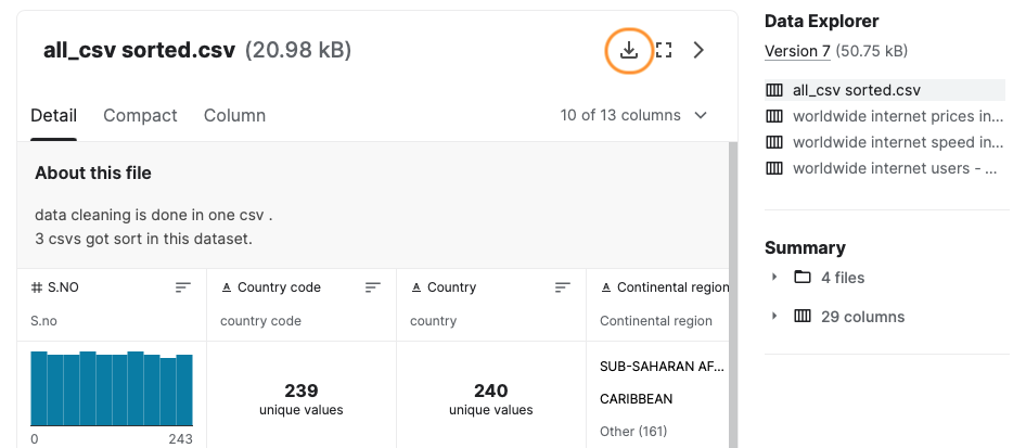
At the time of writing this chapter (Aug. 14, 2022), there are four datasets available. We are particularly interested in ‘all_csv sorted.csv’ (version 7 at the time of writing). This dataset combines the other three datasets into one larger dataset with 200 rows and 13 columns. The file contains data on the average, minimum and maximum price of 1 GB of data in 2022 and the averages in the two previous years (if available). You will also find the number of internet users and residents in each country and the average speed of a connection in Mbit/s. As already mentioned and yet important: we have no idea where the data comes from, so use this data with caution.
Download this dataset via this direct download link to the CSV file.
Possibly this dataset will then just open in your browser window. Either you explicitly command the linked file to be downloaded , or select the entire contents of your browser window (Win: CTRL + A, Mac: CMD + A) and copy and paste this content into a new text file.
Save the file as ‘internetprices.csv’.
CSV files
A CSV file (‘Comma Separated Values’) is an ordinary text file that is useful to exchange data between different applications. For example, you can export an Excel file in this format. Between each column value there is a separator (which you can often choose yourself) such as a comma, semicolon, etc. Each row starts on a new line. The downloaded file looks like this:
S.NO,Country code,Country,Continental region,NO. OF Internet Plans,Average price of 1GB (USD),Cheapest 1GB for 30 days (USD),Most expensive 1GB (USD),Average price of 1GB (USD at the start of 2021),Average price of 1GB (USD â€" at start of 2020),Internet users,Population, "Avg
(Mbit/s)Ookla"
0,IL,Israel,NEAR EAST,27,0.05,0.02,20.95,0. 11,0.9,"6,788,737","8,381,516",28.01
1,KG,Kyrgyzstan,CIS (FORMER USSR),20,0.15,0.1,7.08,0.21,0.27,"2,309,235","6,304,030",16.3
2,FJ,Fiji,OCEANIA,18,0. 19,0.05,0.85,0.59,3.57,"452,479","883,483",25.99
3,IT,Italy,WESTERN EUROPE,29,0.27,0.09,3.54,0.43,1.73,"50,540,000","60,627,291",37.15
…
The first line of a CSV file usually contains some sort of column header, in this case:
- a number (type of serial number),
- two-letter country code,
- name of the country,
- region,
- number of different internet formulas,
- average price of 1GB,
- cheapest price for the same,
- most expensive price,
- averages for both previous years,
- number of internet users,
- number of residents,
- average data rate.
Since this is a text file, you can open, view and manipulate it with an editor. You choose which editor you use for this, but in this example we'll use Visual Studio Code (‘VS Code’), an editor that you undoubtedly use in other courses (frontend, programming, …) as well. Proposal: install in VS Code the extension ‘Edit CSV’ created by a certain janisdd. This extension allows you to work in a spreadsheet-like representation with rows and columns to view the data and manipulate it.
A second useful extension for CSV files is ‘Rainbow CSV’. This gives the different columns a different color and makes them therefore easier to distinguish from each other. Also install this extension in VS Code.
The two screenshots below show the original CSV file without and with the extension ‘Rainbow CSV’. The colored version is a lot more readable, isn't it?
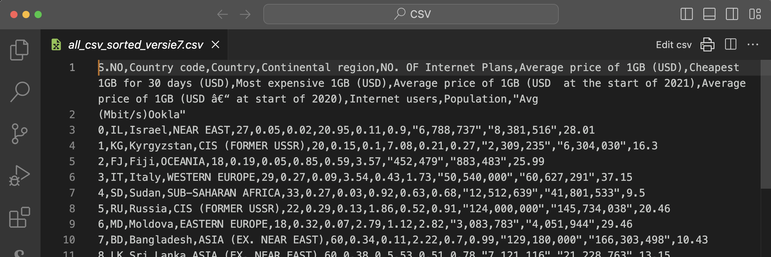
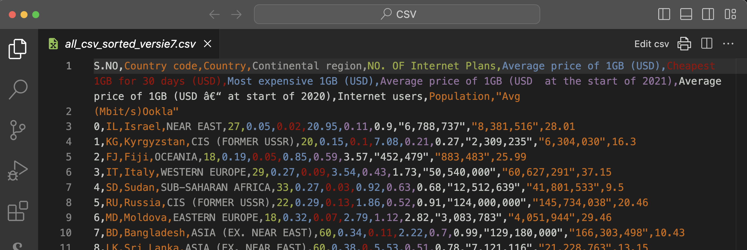
Attention: there is a small error because there is an ‘enter’ between ‘Avg’ and ‘(Mbit/s)Ookla’. Be sure to remove that so that the full header is only on the first row!
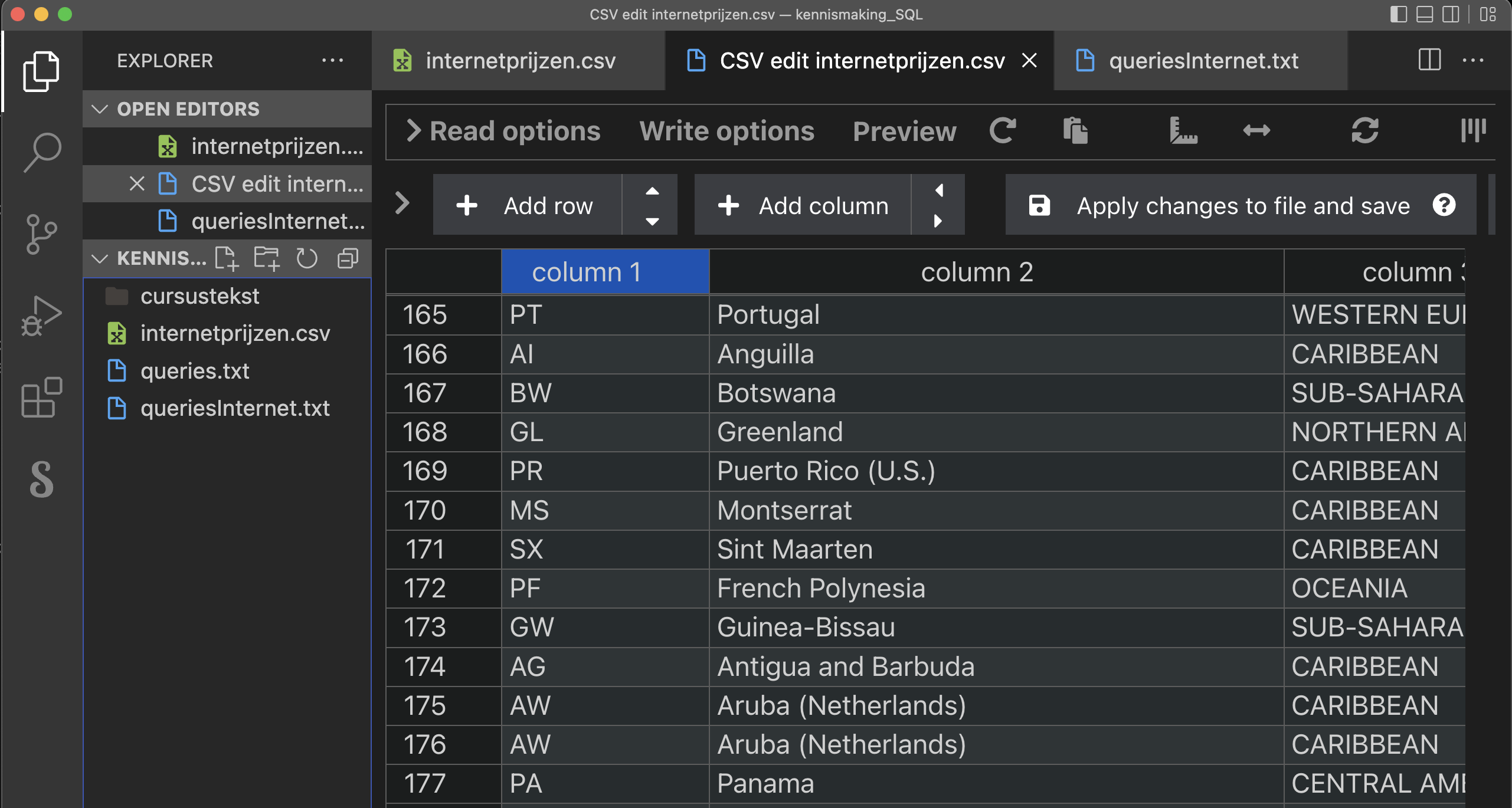
Once these extensions are installed, open the csv file and click ‘Edit CSV’ in the upper right corner. You now get the following presentation of the file:
Data cleaning
A dataset is rarely usable without modification. This dataset also contains some annoying things that make it difficult to load into a table.
Unnecessary columns
You can only load CSV data into a existing table. So you have to first create a new table. You already know that every table has a primary key: a field (or combination of fields) that is unique to each row. The first column from this dataset contains an incremental integer (we'll later call this a ‘technical key’). This could certainly serve, but let's look further.
The second column contains a country code consisting of two letters. That country code is guaranteed to be unique if it follows the standard. Actually, it is then a better idea to use this second column as the primary key for our table .
The first column actually contains useless information. It is best removed from the file. The extension ‘Edit CSV’ that you installed in VS Code makes this easy. If you have not done it before, just click ‘Edit CSV’ in the top right corner. You then get a column view of the file. Hover over the header ‘column 1’. A trash can icon will appear. Click it to delete this column.
Character encoding
Scroll to row 35. I don't know what it will look like on your screen, but on my Mac I read "Réunion" as the country name. That's a typical problem with the character encoding. To make a long story short: computer makers have (long ago) agreed on which combinations of bits correspond to which letter, digit, character. If you don't use the same character encoding as the one used for this file, certain letters will be misinterpreted.
The most commonly used character encoding is UTF-8. That is the standard encoding of your browser, of VS Code, ... Also in a database server, you can choose your character encoding. Let's agree that we will always choose UTF-8. There are some country names that contain special characters such as é, ô etc. Let's modify those manually. If you have trouble finding those characters on your keyboard, you can always copy them from a file that does have those characters correctly.
Adjust the following (unless they are already correct):
- row 35: Réunion
- row 125: Saint Barthélemy (St. Barts)
- row 131: Côte d'Ivoire
- row 139: a difficult one, a swedish capital letter: Åland Islands (it's probably easiest to copy the letter from here)
- row 199: Curaçao
- and finally the most difficult one on row 229: São Tomé and Príncipe.
With that, this bit of the ‘data cleaning’ is done. We can still wonder if we need the first row. In principle we do not, but it contains useful info that is needed to define the table later. Moreover, we can indicate later during import that the first row should not be be imported.
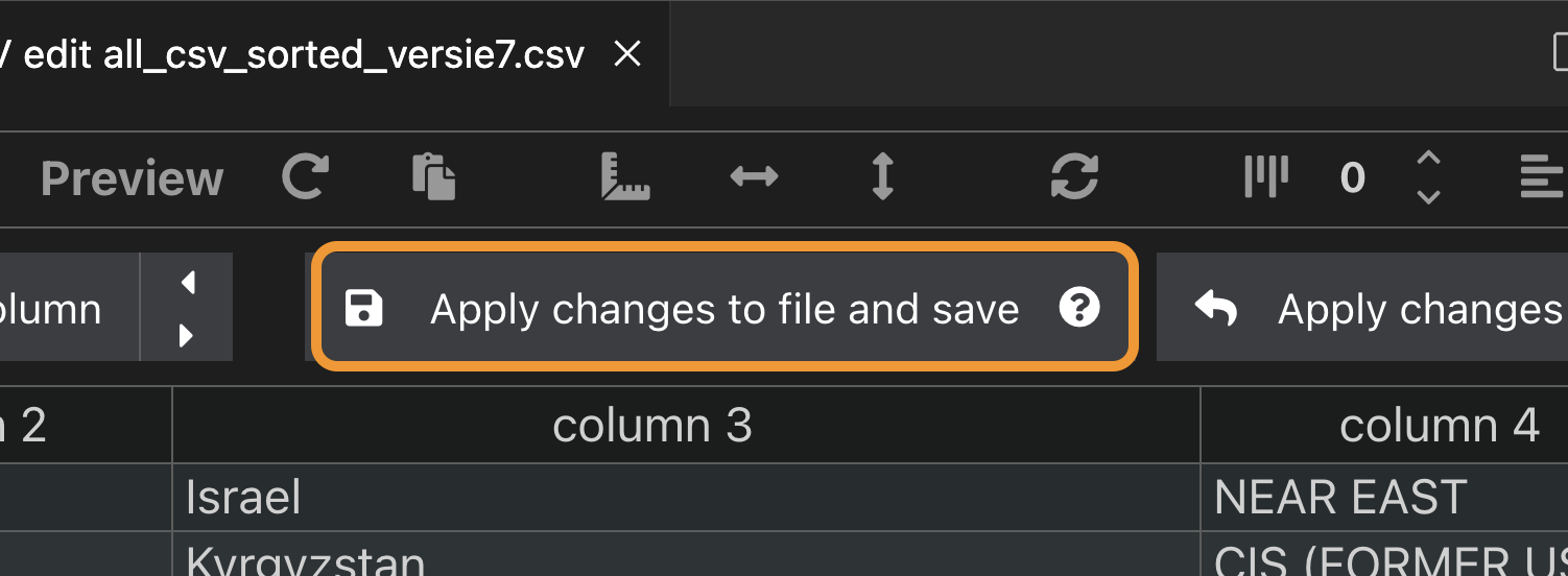
To be on the safe side, save these changes to VS. Code: ‘Apply changes to file and save’ (see screenshot below).
Missing info
From row 233 (‘Christmas Island’) onwards a lot of information is missing: either there are no providers, or the currency in which costs are expressed is so unstable that it cannot be converted into dollars. Let's remove all these rows (i.e., from ‘Christmas Island’ to ‘Zimbabwe’) from this example. You can do that in the column version, but actually it's simpler in the text version because in the column layout you have to do it row by row.
Go over everything again. Here and there the description ‘NO PACKAGES’ stands out. These are often tiny countries. Let us remove rows from the dataset as well. More specifically the following five countries (rows) may be removed: ‘Cook Islands’, ‘Vanuatu’, ‘Tuvalu’, ‘Cuba’ (bit of a shame because this is a big country after all) and ‘Cocos (Keeling) Islands’. Now delete these rows (best in the text version, do a search for ‘PACK’) and save the file one last time.
I want to add a word of caution here. In real-world situations, deleting or altering data can have serious consequences for the validity of your study. For example, imagine you are analyzing the median income in Belgium. People with lower incomes may be less willing to disclose their monthly salary. If you simply delete those missing responses, your results could show a median income that is significantly higher than reality. You will learn more strategies for handling missing data in future classes. For now, remember: when working with real data for a real client, always ask questions before deleting or modifying data. .
Different number notation
Notice that the large numbers representing residents and users use the US notation: thousands are separated by a comma while the separator between unit and decimals here is the period and not the comma. That period is not a problem, but the comma between numbers is going to be a problem when importing the data . We just want the numbers and no separator for thousands, millions, etc.
This is complicated by the fact that we cannot simply omit all commas, because that comma is also the separator between the different columns. And I must honestly admit that in preparing this teaching text, I spent quite a bit of time fiddling with Excel. That was my first plan: import this data into Excel, edit it there and then export it back as a CSV. Sounds very simple, but the process was rather frustrating.
The best thing you can do if it doesn't work is to take a walk ...

When I came back I suddenly saw that it really could easily be done in VS Code itself . The impetus for a solution is in one of the previous paragraphs. Now execute the following steps in VS Code:
The separator between columns is the comma. A CSV file can use other characters as separators, however. We can set this through the VS Code extension. So again, choose ‘Edit CSV’. At the top of the window you have ‘Write options’. In the write options, choose as the separator (‘Delimiter’) the semicolon ‘;’). Apply and save via the ‘Apply changes to file and save’ button. Close both .csv files (the original and the ‘edit CSV’) in VS Code and open the original .csv file again to view the modification. The CSV file now uses the ; between two columns:
Country code;Country;Continental region;NO. OF Internet Plans;Average price of 1GB (USD);Cheapest 1GB for 30 days (USD);Most expensive 1GB (USD);Average price of 1GB (USD at the start of 2021);Average price of 1GB (USD at start of 2020);Internet users;Population; "Avg (Mbit/s)Alsola") Israel;NEAR EAST;27;0. 05;0.02;20.95;0.11;0.9;6,788,737;8,381,516;"28.01"
KG;Kyrgyzstan;CIS (FORMER USSR);20;0.15;0.1;7.08;0.21;0. 27;2,309,235;6,304,030;"16.3"
FJ;Fiji;OCEANIA;18;0.19;0.05;0.85;0.59;3.57;452,479;883,483;"25.99"
…
The only commas left now are those between thousands, millions, etc. So those can be removed with a search/replace command in VS Code (see figure below).
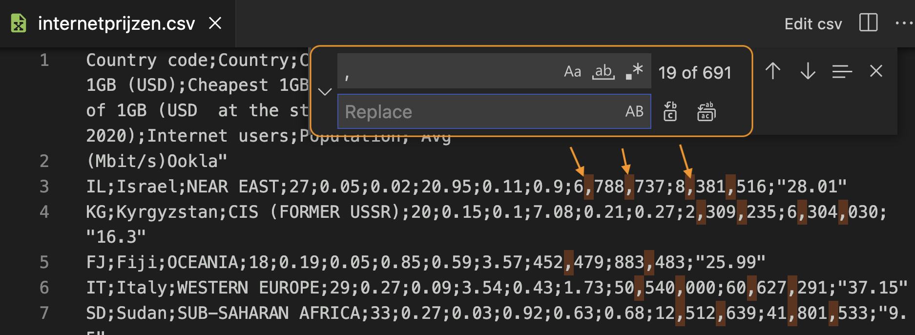
In the search field enter the comma, leave the replace field empty (not even a space). The buttons on the right hand side allow you to substitute one by one or all at once. In the text itself you can see all commas that will be removed. That looks good, so just do all at once. If it goes wrong, don't panic: Undo!
The double quotes ("...") around some numbers should also be removed. After all, we want to read this data into the database as a number because we want to preform calculations with those numbers. So they should not be read in as strings.
Remove all double quotes with a search/replace command in VS Code via Edit > Replace.
After removing these two characters, the end result looks like this:
Country code;Country;Continental region;NO. OF Internet Plans;Average price of 1GB (USD);Cheapest 1GB for 30 days (USD);Most expensive 1GB (USD);Average price of 1GB (USD at the start of 2021);Average price of 1GB (USD at the start of 2020);Internet users;Population;Avg (Mbit/s)AlsolaNIL;Israel;NEAR EAST;27;0. 05;0.02;20.95;0.11;0.9;6788737;8381516;28.01
KG;Kyrgyzstan;CIS (FORMER USSR);20;0.15;0.1;7.08;0.21;0.27;2309235;6304030;16. 3
FJ;Fiji;OCEANIA;18;0.19;0.05;0.85;0.59;3.57;452479;883483;25.99
IT;Italy;WESTERN EUROPE;29;0.27;0.09;3.54;0.43;1.73;50540000;60627291;37.15
SD;Sudan;SUB-SAHARAN AFRICA;33;0.27;0.03;0.92;0. 63;0.68;12512639;41801533;9.5
RU;Russia;CIS (FORMER USSR);22;0.29;0.13;1.86;0.52;0.91;124000000;145734038;20.46
MD;Moldova;EASTERN EUROPE;18;0.32;0.07;2.79;1.12;2.82;3083783;4051944;29.46
…
The file is now ready to be imported into a table. So let's create that table now.
Create schema and table via pgAdmin
Via pgAdmin you already have access to a schema with your student number ‘rxxxxxxxx’ as name in the database belonging to your class. In this schema we will now create a new table ‘internet prices’ (you can create as many tables in your schema as you want). Let's go through all of the columns:
-
The country code (column 1) is a two-character string, so
char(2). It is required because it will be our primary key. -
The name of the country (column 2) and the region (column
3) are indeterminate in length. So those will need to be
varchar(). Choose for yourself the number of characters for both that is sufficient to store all the names (look for the longest string). Both are mandatory. -
The number of internet formulas (column 4) is a small integer. The
data type
smallintcertainly suffices. Also a required field. -
The next three columns are average price, minimum price and
maximum price for 1 GB of data. These are required fields that represent
a dollar amount. A suitable data type for this is
numeric(5,2). In this, 5 is the total number of digits and 2 is the number of digits after the decimal point (i.e., an amount rounded to 1 dollar cent). All three values are indicated each time in the dataset. -
Columns 8 and 9 are average prices of the two previous years.
There too, the choice of
numeric(5,2)is fine. There is a small problem if you look at the dataset. These numbers are not specified for each row. So here we are not going to add the requirement ofNOT NULL. These fields may well be left blank when importing the data. -
Columns 10 and 11 are the number of internet users and the
number of residents
. These are large integers, so
integeris an appropriate data type. Check if all rows have this info. If they do, then you may require that these fields cannot be left blank. -
Finally, the last column is another one that is not always known, namely
the average data rate. Again, this could be a
numeric(5,2)probably.
Now, as an exercise, create this new table with a CREATE
statement. Some typical errors that often recur:
- You are accidentally working in the schema ‘Public’ (explanations and solutions).
- You use column names with spaces: bad idea. In itself it can be done, but then you should always enclose the name in double quotes ("..."). A better solution is to write words together or use a low dash (underscore).
- You forgot to define a primary key.
CREATE SCHEMA u0012047; -- probably unnecessary because this schema exists already
SET search_path to u0012047; -- otherwise you're working in schema public!
CREATE TABLE internet_prices (
  country_code         char(2) NOT NULL,
  name                 varchar(60) NOT NULL,
  region               varchar(50) NOT NULL,
  number               smallint NOT NULL,
  avg_price            numeric(5,2) NOT NULL,
  min_price            numeric(5,2) NOT NULL,
  max_price            numeric(5,2) NOT NULL,
  avg_21_price         numeric(5,2),
  avg_20_price         numeric(5,2),
  internet_users       integer,
  residents            integer,
  avg_data_rate        numeric(5,2),
  CONSTRAINT pk_internet_prices PRIMARY KEY ( country_code )
);
CSV import via pgAdmin
CSV is often used to exchange data between applications. It is therefore obvious that a PostgreSQL database server can work with CSV files. The client we are using (pgAdmin) allows us to perform this operation easily.
About that ‘simple’ perhaps a small warning ... When importing a CSV file into a table you will almost certainly run into some errors. Sometimes a column definition is not quite compatible with the data or the CSV file still contains small errors, etc. We hope that the cleanup operation we did above will be sufficient to make the importing succeed.
False hope, as we will soon see ...
The import is done in pgAdmin as follows. Right click on the name of the newly created table and choose ‘Import/Export Data... ’. In the dialog box (tab ‘General’) you now set the following:
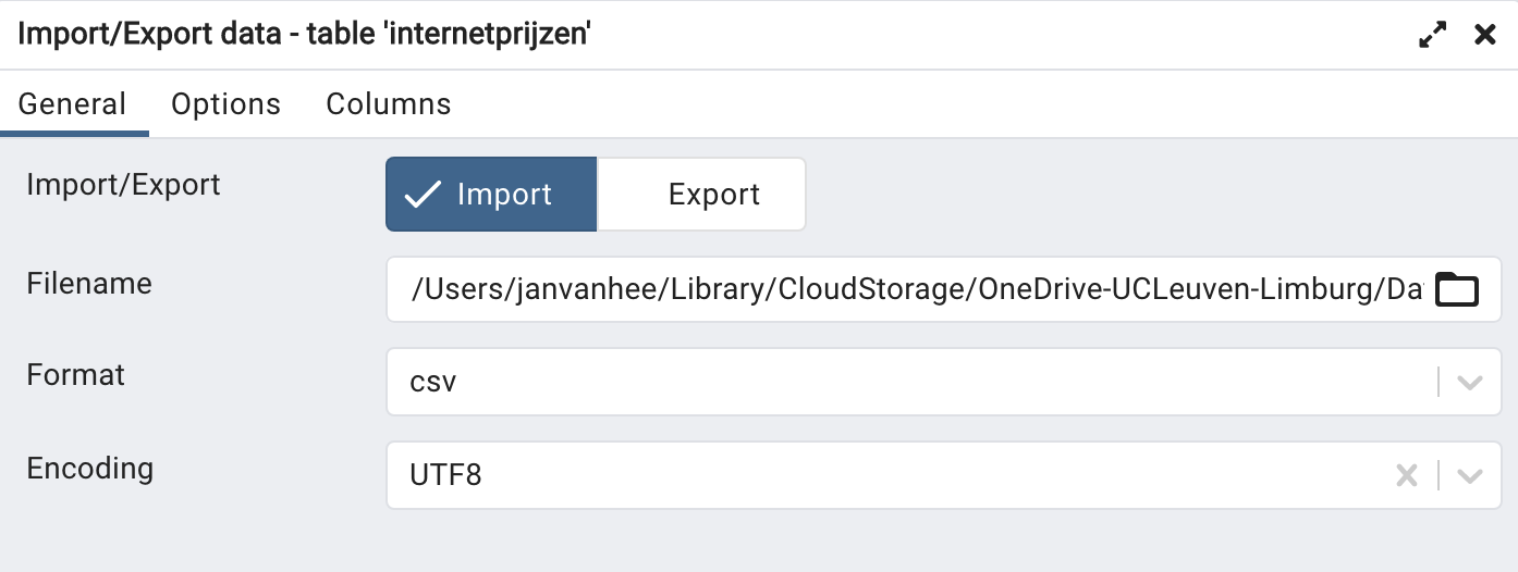
- Import/Export: select Import;
- Filename: link to the .csv file you want to import (‘internetprices.csv’);
- Format: csv;
- Encoding: UTF8;
In the second ‘Options’ tab (figure below), adjust the following:
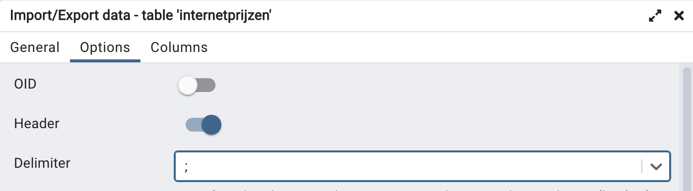
- Header: checkbox (so that the first row is skipped);
- Delimiter: choose ‘;’ as separator;
- You don't need to change the rest of the options.
Confirm with OK. If all goes well, all the rows of the CSV file are now read into rows of the table.
But as mentioned ... things rarely go quite as planned the first time. We thought our ‘data cleaning’ was successful, but you still get an error message. To see this error message, you must first go into the red box where there is an error message, click on ‘View Processes’. You will then get a table with a line of information about the failed import process. In that line, just before the ‘PID’ column there is a ‘View Details’ icon. Click it to see the correct error. You may need to enlarge the window to read the full error message. Such an error message will look like this:
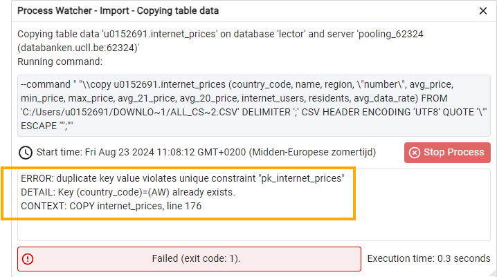
Apparently, the country code AW (our primary key!) appears twice around line 176 of the CSV file. Since the primary key must be unique, the database server rightly gives an error message and the import is aborted. Therefore, nothing is imported.
Look near that line in the code:
...
AG;Antigua and Barbuda;CARIBBEAN;39;4.44;1.48;42.18;7.17;12.7;77529;96286;
AW;Aruba (Netherlands);CARIBBEAN;17;4.44;0.74;8.96;9.11;5.56;15877494;17059560;108. 33
AW;Aruba (Netherlands);CARIBBEAN;17;4.44;0.74;8.96;9.11;5.56;102285;105845;108.33
PA;Panama;CENTRAL AMERICA;8;4.49;2;7.48;6.69;4.69;2371852;4176869;17.03
...
So there are two countries with country code AW and the same name Aruba. A quick visit to Wikipedia reveals that Aruba has just over 100 000 inhabitants. That number corresponds to the second line. The first line presumably corresponds to the Netherlands, as it has about 17 million inhabitants. Let's look at the data of the Netherlands in the CSV file to confirm our thoughts. Through a search in VS Code we find the following:
NL;The Netherlands;WESTERN EUROPE;24;3.11;0.77;15.97;2.98;4.62;;;So this line is missing the number of internet users, the number of population and the average speed. We warned in advance about the lack of clear source citation for this dataset. Now it also appears that there are errors in the file. Presumably the error is best corrected by moving the data from the first entry of AW, Aruba, ... to the line about the Netherlands and then removing that first line from Aruba from the file.
NL;The Netherlands;WESTERN EUROPE;24;3.11;0.77;15.97;2.98;4.62;15877494;17059560;108.33
...
AG;Antigua and Barbuda;CARIBBEAN;39;4.44;1.48;42.18;7.17;12. 7;77529;96286;
AW;Aruba (Netherlands);CARIBBEAN;17;4.44;0.74;8.96;9.11;5.56;102285;105845;108.33
PA;Panama;CENTRAL AMERICA;8;4.49;2;7.48;6.69;4.69;2371852;4176869;17.03
...
Next attempt. Repeat the import steps. This also goes wrong because country code LB appears twice. The CSV file reads:
LB;Lebanon;NEAR EAST;15;4.81;1.21;77.7;3.82;5.84;4755187;6859408;16.38
LB;Lebanon;NEAR EAST;15;4.81;1.21;77.7;3.82;5.84;4755187;6859408;16.38
This error is simple to correct: delete either line in VS Code. Don't forget to save your file afterwards!
New attempt. Fortunately, this time we get the message that the import was successful via a green window with ‘Process completed’.
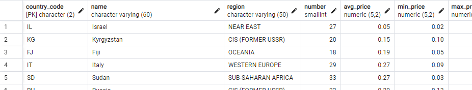
Request a complete overview with SELECT * FROM internet_prices:
From data to information
We have put the data (a collection of facts) into a table. Now we can use SQL to structure this data, combine it, organize it differently, etc. Remember that we talk about converting data to information.
By way of example, let's look for an answer to the question of how Belgium compares to other countries in terms of cost (in 2022) of 1 GB of data on the internet. This can be found with the following simple query:
SELECT name, avg_price
FROM internet_prices
ORDER BY 2; --so from cheap to expensive
Test this and subsequent queries yourself!
Belgium is ranked 186 according to this data. Our internet connections are expensive!
So where do we stand compared to our neighbors in Western Europe? There too we are not doing so well. Only three countries (Norway, Andorra and Greece) are even more expensive than Belgium, as the following query shows:
SELECT name, region, avg_price
FROM internet_prices
WHERE region ='WESTERN EUROPE'
ORDER By 3;
Exercises on this dataset
The best way to learn about a dataset is to play with it. Test different queries. Try to solve the following exercises.
Ranking based on internet speed
Create a ranking of all countries based on average data rate. The country with the fastest connection should be at the top. Display only the columns ‘name’ and ‘avg_data_rate’. In a second version of this query show only those countries for which a rate is given.
A first version of the query could be this:
SELECT name, avg_data_rate
FROM internet_prices
ORDER BY avg_data_rate DESC;
You'll notice something special in the output: all rows containing NULL in the rate column are shown first. This is because for PostgreSQL
NULL values are considered larger than all non-NULL values. This behavior depends on the database: Oracle does it the same
way, but SQLite and MySQL do it the other way around. Those database servers
consider
NULL as a value smaller than all other values.
To display only those rows for which there is effectively a rate
given, you can filter for the value NOT NULL:
SELECT name, avg_data_rate
FROM internet_prices
WHERE avg_data_rate IS NOT NULL
ORDER BY avg_data_rate DESC;
Country with most expensive average price
Which country has the most expensive average price for 1 GB of data?
SELECT *
FROM internet_prices
ORDER by avg_price desc;
Biggest price difference
In a SELECT, you can also count with columns. We
will make use of this in this exercise.
In which country is the price difference between the most expensive and the cheapest offer the greatest? (Answer: Greece, where the difference is so large that you have to wonder if these numbers are correct ...). You should obtain the screenshot of the figure below.
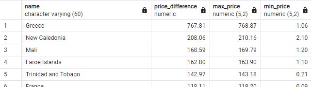
SELECT name, max_price - min_price AS price_difference, max_price, min_price
FROM internet_prices
ORDER BY 2 desc;
Country in the Americas with fastest internet
Which country on the American continent (both North and South America) has the fastest internet speed? Create an SQL query that will generate a list where you can find the answer.
This is already an extended combination of AND and OR. Don't worry if you find this difficult, we will come back to this
in the next chapter.
SELECT name, avg_data_rate, region
FROM internet_prices
WHERE (region = 'SOUTH AMERICA' OR region = 'NORTHERN AMERICA') AND avg_data_rate is not null
ORDER BY avg_data_rate desc;
Percentage of internet users
This is a difficult exercise!
Calculate the percentage of internet users of each country and rank them so that the country with the largest percentage is at the top. In case you thought until now ‘Surely everyone in our country has internet access?’: Belgium has a percentage of 87% ... Below in the solution some tips, but first try the exercise without the tips!
- A percentage is the number divided by the total number multiplied by 100.
-
There is a problem with the division of two integers. Try the following code:
SELECT 1 / 2;This division produces a surprising result: 0. The reason is that this is a whole division. The number 2 effectively goes 0 times into 1. Try a few other number combinations until you understand how integer division works. If you want to obtain a float (decimal) as a result, you must use the
CAST ... AS ...operator. Type the followingSELECT:SELECT cast(1 AS float) / cast(2 AS float);This
SELECTcalculates the division of two decimal numbers. The result is now also a decimal number, which is called a float in the database. - We don't want
NULLvalues in the output. -
Make use of an alias (with
AS) in theSELECT.
This code is a good solution:
SELECT name, cast(internet_users as float) / cast(residents as float) * 100 AS percentage
FROM internet_prices
WHERE internet_users / residents is not null
ORDER BY 2 desc;
Grouping data with GROUP BY
Now that we have a sufficiently large data set, we can group
(or with a technical term ‘aggregate’) data in a meaningful way,
e.g., by region. We
introduce the GROUP BY for this purpose. A thorough treatment
follows in the chapter ‘GROUP BY / HAVING’.
Order in which a query is executed
By now you can already create simple queries. Those queries are completed by a database server in this order:
-
FROM: which table(s) do we need and should be loaded into memory? WHERE: which rows of these tables do we select?SELECT: which columns do we display in the result?-
ORDER BY: according to which column(s) are the rows ordered in the result?
Note that this is different from the order in which you write the query!
Grouping data
Sometimes you no longer want to retrieve individual details, but are only interested in information about a particular group. Some examples for the table of internet prices:
-
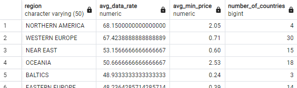
What is the average internet speed, average minimum price and number of countries in each region (see figure)?
-
List the countries by the number of internet formulas (from at least 40 formulas) and give the average price:
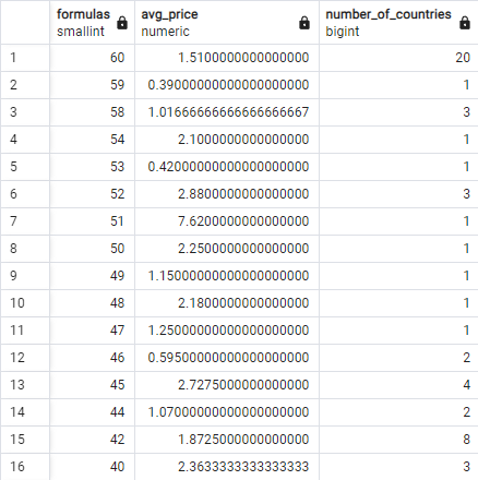
Let's solve the question from the first example: “For each region, list the
number of countries in that region, the average internet speed and the average
minimum price.”. We need to provide some information by region so we use GROUP BY region. At this point we can only retrieve the region itself and summary numbers (aggregation functions applied to certain columns). This gives the following query:
SELECT region, AVG(avg_data_rate), AVG(min_price), COUNT(*)
FROM internet_prices
GROUP BY region
ORDER BY 2 DESC;
Let's go through the execution of this query step by step in the correct order (i.e., not the order in which the query is written!):
-
FROM internet_prices: the entire table internet_prices is loaded into memory. - There is no
WHERE, so no rows are dropped. -
Next comes the
GROUP BY region: all rows with the same region end up in one box. On each box, the name of region will appear. So there will be as many boxes as there are different regions in the table. -
Only now is the
SELECTexecuted. The only thing we can now retrieve is the label of each box (region) and summary information of all the data contained in each box using aggregation functions such asAVG(avg_data_rate)(arithmetic average of all rates in each box),AVG(min_price)(arithmetic average of all min prices in each box) andCOUNT(*)(the number of rows in each box). -
Finally, the rows in the final result are ordered (
ORDER BY 2 DESC) from large to small according to the second column so that the row with the largest average speed is at the top.
Classical error with a GROUP BY
Take a look at the following simple query. This query will fail because it contains errors. What is wrong with it?
SELECT *
FROM internet_prices
GROUP by region;Read carefully the error message you get:
ERROR: column "internet_prices.country_code" must appear in the GROUP BY clause
  or be used in an aggregate function
LINE 2: select *
               ^
SQL state: 42803
 Character: 39
Using the GROUP BY, all rows with the same value for the
field ‘region’ are put into one box. From this box you can only select the
name (‘region’) and averages, maxima, minima, number and sum
(the five aggregation functions) of some columns. With SELECT * you query all columns, which cannot be done. It immediately
goes wrong with the first column (‘country_code’), hence the message that this
column must be in the GROUP BY.
HAVING
In a query with GROUP BY, you will also regularly encounter a HAVING. This is somewhat similar to a WHERE in that it also makes a
selection and possibly causes data to drop out. Consider the following example:
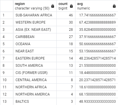
SELECT region, COUNT(*), AVG(avg_data_rate)
FROM internet_prices
GROUP BY region
ORDER BY 2 DESC;
This query lists by region the number of countries in that region and the average internet speed in that region. The following figure shows the full results, arranged descending by the second column:
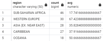
We can now add a HAVING in the code:
SELECT region, COUNT(*), AVG(avg_data_rate)
FROM internet_prices
GROUP BY region
HAVING COUNT(*) > 16 --has to come after the GROUP BY clause
ORDER BY 2 DESC;
The addition of HAVING COUNT(*) > 16 means ‘keep only those
boxes (regions) that contain more than 16 individual rows’. The result of the
query now consists of far fewer rows:
So what is the biggest difference from WHERE? The WHERE is executed right after the FROM and before the GROUP BY comes into play. The condition behind WHERE selects certain
rows of the table (and discards the others). Only then are these rows collected
into boxes collected by GROUP BY. Only when every row is in a
box, the HAVING is started which keeps certain boxes and removes
others.
The various statements in a query are executed in this order:
FROM: which tables contain the info?-
WHERE: which rows satisfy the condition? Retain only those rows. GROUP BY: do we put info together in boxes ...?HAVING: ... that meet a certain condition?SELECT: which columns do we display?ORDER BY: how are the rows ordered?